Laboratory Schedule for 2007, Biology 164

Note: labs may be rescheduled to respond to experimental difficulties or opportunities.

Labs will be in Seaver West basement, room 007, from 1:15-5:00 Weds afternoons, and possibly longer at times, with 1-3 hours outside of laboratory periods in some weeks.

The purpose of the laboratory of Bio164 is for the class to study genetic regulation in the eukaryote budding yeast.  The class as a group will design experiments, carry them out, generate original data, and make conclusions concerning a specific system they have chosen to investigate genetic regulation in yeast.  The yeast genome is completely sequenced and around 6000 genes have been identified.  They include a number that appear to be ORFs  (Open Reading Frames) but may or may not actually encode anything.  All yeast ORFs have an ID number that assigns them to a place on a chromosome and the Watson or Crick strand for the mRNA sense strand.  Most also have a gene name that represents what we know of the function of the gene.  Much information about each gene is collected and accessible via the Saccharomyces Genome Database at Stanford.  The web site, which you will be accessing frequently for this laboratory, is:    http://www.yeastgenome.org/

Microarray analysis enables us to examine the expression of all of these ORFs at once, in response to an environmental or mutational change.  We can thus get a view of compensatory regulatory changes that is much more comprehensive than is available in most organisms.  We can see if entire pathways change, if many genes involved in one organelle are changed, and many other kinds of integrative change patterns are possible to detect.   The class will choose a regulatory question to study using this method.  We can get background data and access to relevant literature via the Stanford Microarray Database at:

http://genome-www5.stanford.edu/MicroArray/SMD/

The second method we will use is quantitative Reverse Transcription PCR.  This method enables one to examine the expression of a single gene in comparison with a standard gene known not to change in expression, in two different RNA samples.  The mRNA present is copied into cDNA and a variety of dilutions and replicates enable one to obtain its efficiency of amplification and its amount of amplification compared to our standard gene, TUB1.   The real time PCR machine (ABI Prism 7000) will be used with SYBR Green dye and a denaturation analysis following the PCR step for this analysis.   The part of the laboratory procedural notes  giving procedures for qRT PCR will be handed out later in the semester.

The third method we will employ will be fluorescent microscopy of Green Fluorescent Protein-Labeled Proteins.  We will use GFP-Hsp12, a membrane protein that is strongly induced by stress, and GFP-Msn2, a stress-related transcription factor.  Msn2 is controlled by phosphorylation, which keeps it in the cytoplasm.  We will use these marked proteins to observe effects of whatever stressor is chosen by the class as subject of your investigation in 2008.

The laboratory performance will be graded by LH based on her observations of your seriousness of purpose and thinking in lab (mistakes don't affect your grade unless you seem to be making mistakes because you are not paying close attention.  The grade will be based upon a laboratory notebook that will be graded twice during the semester.  Use your lab notebook in preparation for and during every laboratory as a journal of what you will do/are doing.  Lab books should include background material with references for each of the experiments, including reading and description of both the concepts and the methods used.  They should also reflect everything you have done and when it was done, and provide enough information to allow someone else to repeat your experiment.  You should include the laboratory handouts by pasting them in if you are using a bound notebook,  or by including them as pages if you are using a loose leaf notebook.  Make sure your lab notes reflect that you have read and assimilated the laboratory handouts.  Also, make sure you have analyzed and commented upon each result, whether control or experiment in nature.

Jan 23, lab 1.  LH discusses with class the possible projects for the year.  Next week, students choose to study a particular stress such as UV irradiation, heat shock, or glucose exhaustion in the medium during growth (the whole class will study one of these).  We will read and discuss papers on each of these and decide on the topic at the second laboratory session.  Today, you will be formed into two or three groups and given background materials to read and prepare for next week's laboratory.  Today, we will also read two papers on microarrays handed out in laboratory and discuss microarrays as a technique (what are they?  what kinds of questions do they help us to address?  what are their limitations or problems?)  During lab, you should take some notes on these issues in your laboratory notebook.  Action items for between laboratories: Before lab, get instructions for logging into the GCAT assessment site and taking the pre microarray survey there.  Between labs, read the papers assigned for your group and plan an experiment to present to the class.

Jan 30, lab 2.  LH and students discuss the potential student selected group project and choose one of the experiments by a secret ballot vote.  Students take notes on the presentations in lab notebooks.  After the vote, class discusses any changes that might be considered for the proposed experiment, and plans are made for preparing the samples needed.  Students from the group proposing a different project receive the background readings for the project that has been selected, and should take notes on them between labs.  LH describes software for class: MagicTool, BRB ArrayTools, GenePix, and GeneSpring.   Then, the class will go to SW014, Hoopes' research lab,  and be introduced to using the software for microarray analysis. Action items: Write up tentative hypotheses in lab notebooks using notes and materials given out.   Be sure to predict changes in specific genes in your notebook, based on hypotheses.

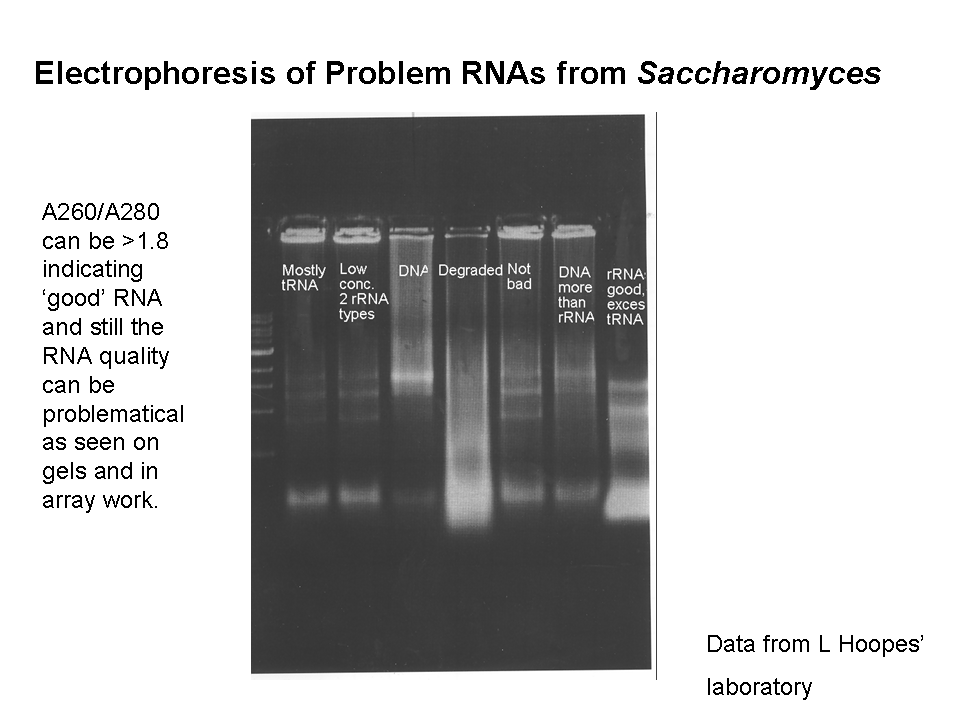
Feb 6, lab 3.  LH introduces the day’s experiment briefly. Treatment of cells as planned and isolation of RNA; see lab handout; add handout to notebook.  Use RNA paranoia!!  Be sure to note any deviation from written procedure in your lab notes.  We will begin with total RNA rather than mRNA in our experiment, so we will not isolate polyA+ RNA.     Action items: examine the handout on RNA quality assessment in gels and be ready to interpret your results next week.  Read over the RNAa procedure since you may do step 1 next week in laboratory.  Take notes into your lab notebook from SGD web site on two specific genes you predict might change in our expression in our experiments.

Feb 13, lab 4.  LH calls on two students to review the purpose of the experiment and what was done last week.  This week's lab: quality control tests on the RNA prepared and if high quality, first strand and second strand cDNA synthesis.  LH describes the procedures to be used briefly.  Students will dilute a tiny sample of their RNA for absorbance testing and will also apply another tiny sample of it to an agarose gel for quality control.   While the gel is running, students will practice filtering and clustering data using GeneSpring and the cell cycle data set.  At the end of the period, each pair of students should show the quality control data to Dr. Hoopes and discuss with her whether to go ahead with hybridization or to prepare a new RNA sample next week.  If your RNA is of good quality, then you will begin the amplification of the mRNA to form RNAa.  The remaining total RNA will be frozen for possible future use in RT PCR experiments.  We will conduct first strand synthesis today for 2 hours, then second strand synthesis for 2 hours, and freeze the sample until next week.  Action items: at end of today's lab, we will set up a 2 hour reaction that volunteers can freeze.  Before lab next week, review the steps completed and the continuation of the RNAa protocol.

Feb 20, lab 5. LH calls on two students to review the purpose of the experiment and what has been done so far.  LH describes briefly the continuation of the RNA amplification protocol to be conducted today.  Today, we will purify the cDNA made last week and set it up for RNAa synthesis, incorporating the amino allyl derivative that can later couple with Cy dyes, overnight.  During this laboratory, students will practice gridding spots from last year's data using GenePix and Magic Spot and will practice choosing data for analysis using the cell cycle data in GeneSpring.  Action item: Volunteers are needed to treat it with DNase the next morning, for about 30 minutes,  followed by freezing until the next laboratory.

Feb 27, lab 6.  LH calls on two students to review the RNAa protocol to date.  LH describes briefly the continuation to be completed today and the process of hybridization.  Today we will purify the RNAa that we have synthesized, couple the amino allyl derivative to Cy dyes, quantify it, and hybridize it with microarrays overnight. Action item: Volunteers needed to help wash the microarrays in the morning, and if time permits, to help with scanning.    Be sure to keep your notebooks up to date!

Mar 5, lab 7.   LH calls on two students to review the purpose of the experiment and progress.  LH describes and discuss scanning process and the type of data generated.  Class moves to SW14 at scheduled times (two lab groups can grid at once) and proceeds to grid data with GenePix.  After 1 hour, gridding work must be saved and continued at another time between laboratories, as a new set of groups will be incoming.    After gridding is complete, collect data and save it.  Use a thumb drive to move a copy of your data to the class file on the computer next to the Axon GenePix scanner.  LH will send each student all of the gpr files so they can be imported into GeneSpring for analysis.  Action item: import the gpr files into Excel, extract the columns labeled 'ID' "gene" and 'median of ratios' from the first one to start a new excel file.  Add columns with the 'median of ratios' from each of the other files.  Correct any columns that are from dye inversions by putting in a column of 1/value, which will be equivalent to de-flipping the dyes.  Organize data with ID, gene, and all data, uninverted for all that were dye inversions, next to each other.  Sort by one of the columns and look for interesting patterns of gene behavior.  Note the IDs of 10 interesting genes you found this way in your lab notebook.  Look back in your individual gpr files to see if any of them were for flagged spots (see flag column, if a value appears, it was flagged).  Also look to see if any were from spots with very low intensities (less than 50?  less than 100?) for either or both of the 635 (red fluorescence) and 532 (Green fluorescence) readings.  For any genes NOT flagged or of low intensity, look up the gene on SGD and take notes in your lab notebook on what it was. 

*** Next week at the end of lab, you will be turning in your notebooks for the first grading!  Make sure they are up to date!

Mar 12, lab 8, day after fall break.    During this lab period we will begin the more sophisticated level of data analysis from the microarrays.  Each group should have obtained the gpr files, imported them into GeneSpring, filtered the data, performed ANOVA, and performed one method of clustering by the end of the period.  Take notes in your lab notebook on what you notice during these analyses. This work will continue next week in laboratory.  Action item: turn in lab notebook at the end of the lab period. 

Mar 19, spring break, no lab. 

Mar 26, lab 9  LH will call on two students to summarize the microarray experiment so far.  Lab books will be returned;  continue the data analysis using GeneSpring  and design second gene expression experiments.  Each group needs to have clustered your data using hierarchical clustering (treeview), Kmeans, and  qCLUSTER methods.  You need to record the results of each clustering in a file, and take notes in your lab book of apparent functions represented in the genes seen in each of the clusters. This information needs to be recorded in your lab books, with any thoughts you have about what each clustering method has done.  In your notebook, comment on how the results compare with your hypotheses at different points.    In this laboratory  we will design the second gene expression experiment, capitalizing on the results of the first.  Some students will use arrays again, with dye flips or other kinds of experiments, while others may choose to perform qRT PCR analysis on two genes chosen from the first data set.  For those choosing qPCR, primers must be designed and ordered this week.  Action item: if doing qPCR, have LH verify your primers and plan to do a PCR quality control experiment.  Read handouts on qPCR and be prepared to present next week in lab.

Apr 2, lab 10:  Begin the second microarray or qPCR laboratory work.  Students present material about the technique of  quantitative Reverse Transcription PCR.    LH briefly discusses planned experiments for the day. The students using microarrays for a second experiment will begin RNA preparations needed.    If doing qPCR, your group will do quality control DNA PCRs today to make sure the primers you designed can amplify the right size of fragment, and run a gel on them.  Depending upon the number of groups doing  qPCR, we may run one or two gels.  Make sure to show on the gel diagram where your sample is loaded as well as the gene being tested and the predicted size of the product..  Look at data in the GeneSpring program to see how much our control gene for RT PCR, Tub1, changes its expression in various experiments.  The rest of the time today can be used to follow up on your data analysis from the first set of microarrays.   Action item: quality control on RNA samples.  Between labs, or running late in this lab, someone from each group doing microarrays will need to come in and read the A260/A280 and run a gel on the RNA.  Make sure to share the data with everyone in your group and with LH.

 Apr 9, lab 11.  Begin the cDNA first strand and second strand synthesis if microarray; if RT PCR primers qualified last week if RT PCR experiment, set up and run qPCR.  For microarray groups, today you will run both parts of the cDNA synthesis starting immediately, since quality control has already been completed.  For qPCR groups, set up all RT PCR reactions in one 96 well plate as LH will demonstrate.  Set up a standard curve for each gene and for the standard TUB1.  Set up assays for TUB1 as well as each gene of interest in every RNA sample.  Use triplicate samples.  Use the position chart to locate the wells your samples will occupy.  Run the RT in the ABI Prism, then add the PCR reagents with SYBR green, and run the PCR.  You can watch the real time appearance of data on the computer attached to the Prism. Action item: All students, not just those running the qPCR: get the data set for the qPCR from LH, get the instructions for calculations, and calculate the results.  Write up in lab notebook.

Apr 16. lab 12.  cDNA purification and quantitation, setup RNAa synthesis overnight for microarrays; run second RT PCR for qPCR group.     Those doing microarrays will purify the cDNA and set up RNAa synthesis to incorporate amino allyl derivative overnight. Use directions from previous laboratories.  If doing qPCR, depending on the results from last week we may repeat the same experiment or try some different genes from the list of available primers provided.  Use directions from last laboratory.  Action item: All students, not just those running the qPCR, get data set for qPCR and calculate results, write up in lab notebook.

 Apr 23, lab 13.  Microarray dye coupling, hybridization, washing.  RT PCR third experiment.  For microarrays, continue the procedure as before, coupling the dyes to the activated RNAa and hybridizing with the arrays.  For qPCR, choose one more set of two genes to compare to TUB1, or choose another available RNA to test for some of the genes already examined.  Action items: All students get the qPCR results and calculate; all students get the microarray scans and help to grid them; import the gpr files into excel, and look at data.

Apr 30, lab 14.   In small groups, students observe GFP-labeled stress indicator proteins undergoing stresses relevant to gene expression experiment.  For students not observing on fluorescent microscopes at any particular time, computers available for data analysis.

May 7, lab 15, Data analysis/ work on report on class project.  Using the data posted for microarrays and the qPCR data collected by others in the class, complete the data analysis using GeneSpring, MAGICTool, and ABIPrism7000 software plus Excel for the class project.     Import all of the class microarray data from both sets into GeneSpring and complete the filtering and clustering.  Make notes on how you filtered and clustered (what your settings were and which cluster method you selected) and what you found out.  Save clusters and gene lists; use PIR gene lists to find out what kinds of processes have changed in your tested cells.  Save plots and print a few for your report. OR use MAGICTool and make a correlation matrix and cluster using the various clustering options in that program.  Also, make sure you have analyzed the data from the quantitative PCR experiments done, and related those to the results from the microarray experiments.  Action items: Keep working on Data Analysis. Write up notes on results and conclusions in lab notebook.  Make sure your lab notebook covers all experiments done by the class, whether or not you did them.  Continue data analysis, writing until final deadline (see below).  

May 16. Lab wrap up.  All data analysis must be completed.  Complete lab book handed in by this date. 

Very important: Log into the GCAT site and take the post-microarray survey there. 

2008 Experiment

GenReg Laboratory Group Project Choices for 2008.

Constraints on everyone:

We will only do ONE group experiment in the class, in order to get what we hope will be a significant amount of data addressing our class question.  Each lab group (two students) will be able to do one or two microarray slides (depending upon enrollments) in the first round of experiments.  In the second round,  we will work on verifying the expression of genes identified from the microarray experiments by means of real time reverse transcriptase PCR experiments.  So, plan your experimental tests/controls so that 4 to 6 microarrays will be enough to address your questions/hypotheses.

1.  Stress that Calls for Nucleotide Excision Repair of DNA  

    Background:

Yeast, like most eukaryotic cells, has multiple DNA repair processes.  One of the most important in all kinds of cells is nucleotide excision repair, NER.  In yeast, a complex of two proteins, Rad1p/Rad10p, is a vital part of the NER pathway that makes incisions near a site of DNA damage such as a thymine dimer or other bulky adduct.  Without either of these two proteins, i.e. in strains deleted for either of the two genes encoding the dimer, there is greatly increased sensitivity to UV damage (killing). 

Materials provided for decision making phase: 

1.  Paper that showed just a few genes are induced by DNA damage, regardless of the type of damage (but not including UV damage or looking at a mutant affecting NER):  Gasch, Audrey P. et al, Genomic Expression Responses to DNA-damaging agents and the regulatory role of the yeast ATR homolog Mec1p.  Mol Biol of the Cell 12:2987-3003(2001). 

 2.  Prakash, S and Prakash, L.  Nucleotide excision repair in yeast.  Mutation Research 451:13-24 (2000).  Paper reviews the role of various enzymes in NER process, and shows that complexes exist with the NER proteins associated with other pathway proteins, especially those needed for transcription with RNA polymerase II (TFIIH is a protein that stimulates RNA pol II transcription).  Review article providing background and perhaps ideas about what genes might be affected in NER mutants.  

 Strains available: Wild type W303a; T177, a W303a strain in which rad10 has been deleted and which is therefore deficient in nucleotide excision repair and sensitive to UV irradiation.   Rad1-GFP, Nik1-RFP strain showing where the nucleus is and where this repair protein is in the cell.  Hsp12-GFP showing degree of stress by brightness.  Msn2-GFP showing degree of stress by nuclear location when stress is detected.

 Other information and resources: 

1. The 2003 class tested T177 compared to wild type without UV treatment and found little or no difference in mRNAs assessed via microarrays; this data set is available to be compared with any new data.  Other available data in our lab include microarray data from  wild type/wild type comparisons.  The 2004 class selected this project too, in a close vote, and was able to collect data, but most arrays had one color much stronger than the other and data were not too repeatable.  You may or may not want to include their data in your analysis if you select this project. 

 2.  We have a Stratalinker which can be used to provide UV irradiation to cells on plates.  Cells in liquid don’t receive UV very well, since the water base of the liquid medium absorbs most of the UV energy.

 3. UV damage can be repaired by a photoreactivation system that will reverse the damage; in order to prevent photoreactivation from acting to reverse the DNA damage you have given, you can wrap the container(s) of UV irradiated plates or tubes with aluminum foil to keep out visible light. 

 4.  LH will give the group working towards presentation of this project a survival curve for wild type and for T177 yeast prepared by Adam Simning for his senior thesis; it may be helpful in designing experiments.

2.    Stress in petite strains from yeast.

Background: 

In yeast, if wild type cells are grown on rich medium with ethidium bromide added to it, they tend to lose all or part of their mitochondrial DNA and become respiratory deficient cells that make small colonies (‘petites’, also known as rho minus or r-).  This characteristic is inherited by the progeny cells even when propagated without the ethidium bromide medium.  Since the mitochondrial genome encodes important subunits for some of the electron transport carriers, the electron transport and oxidative phosphorylation reactions cannot occur; the petite cells must grow by fermentation and can grow without oxygen by fermenting glucose to form ethanol. 

Paper 1: Epstein, C. B. et al., Genome-wide responses to mitochondrial dysfunction.  Mol Biol of the Cell 12:297-308 (2001).  Paper shows microarrays of petites and wild types; of course, every time a new petite strain is isolated, there is a chance that a different part of the mitochondrial genome is deleted so there may be differences between his petites and any we isolate here in terms of their gene expression data.  The study suggested an induction of peroxisomes and interaction with the retrograde regulatory genes that participate in mitochondrial/nuclear cross talk in petite strains.  A few different inhibitors and media that would allow only anaerobic or only aerobic growth were tested in this paper; others would be interesting.  For example, what about adding malonate, a competitive inhibitor of an enzyme of the Krebs Cycle, SDH or Succinate Dehydrogenase?  What might that do to gene expression in a petite versus wild type? 

Paper 2: (Not in packet, just for you to know about!) Taylor, D et al.  Conflicting levels of selection in the accumulation of mitochondrial defects in Saccharomyces cerevisiae.  Proc Natl Acad Sci, USA 99:3690-3694 (2002).  Paper cites human degenerative diseases that result from mitochondrial genomic changes, and analyzes mathematically a situation in which defective mitochondria should come to predominate (within- and among-cell selection values were manipulated by the modeling team).  This one is so you will realize the weird ‘petites’ of yeast have potential to help us understand human diseases!

Paper 3: DeRisi, J, Iyer, V and Brown, PO.  Exploring the metabolic and genetic control of gene expression on a genomic scale.  Science 278:680-686 (1997).  Looks at diauxie, which Paper 1 compares with the petite gene expression patterns.

 Strains available: W303a wild type.  You may select new petites by streaking on EtBr plates and choosing tiny colonies for three rounds of streaking.  We may have some strains selected in 2005.

3. Stress in sir2 mutants of yeast. 

Background: Sir2 is a histone deacetylase that is activated by NAD+; it can turn off genes in response to the  metabolic state of the cells.  It exists in a complex of three of the silent information regulator proteins, Sir2, Sir3, and Sir 4, that sits at telomeres and silences any genes in close proximity to the telomeres.  It also is found at the silent mating type loci, and at the nucleolus where the rDNA repeated sequences occur.  Deletions of sir2  have life spans that are about 30% shorter than wild type, while extra copy strains have life spans that are about 30% longer.  This extension is found with one extra copy, but more copies produces shorter life spans.  Sir2 may regulate life span by down-regulating recombination among the approximately 150 copies of the 9kb rDNA sequence. 

Paper 1.  Kaeberlein, M, McVey, M and Guarente, L. (1999) The Sir2/3/4 complex and Sir2 alone promote longevity in Saccharomyces cerevisiae by two different mechanisms.  Genes and Development 13:2570-2580.

Paper 2.  Lin, SJ, Ford, E, Haigis, M, Liszt, G, Guarente, L.  Calorie restriction extends yeast life span by lowering the level of NADH.  (2004) Genes Dev. 18(1):12-6.

Paper 3.  Anderson, RM, Bitterman, KJ, Wood, JG, Medvedik, O, and Sinclair, DA.  Nicotinamide and PNC1 govern lifespan extension by calorie restriction in Saccharomyces cerevisiae.  Nature 423:181-185 (2003).

Paper 4.  Kennedy, B, Gotta, M, Sinclair, D, Mills, K, McNabb, D, Murthy, M, Pak, S, Laroche, T, Gasser, S and Guarente, L (1997) Redistribution of silencing proteins from telomeres to the nucleolus is associated with extension of life span in S. cerevisiae.  Cell 89:381-391.

Paper 5.  Sinclair, D, Mills, K and Guarente, L. (1997) Accelerated aging and nucleolar fragmentation in yeast sgs1 mutations.  Science 277:1313-1316.

Strains available:

W303R wild type, sir2D, SIR2 extra copy, sir2D with hml silent mating type deleted, sir3deletion, sir4 deletion.

 Other resources:

We have microarray data  wild type strains that can provide a basis of comparison for this experiment.

 Experiment chosen:

 LH will fill in after first lab when you choose!

Protocols provided:

Microarray protocol 1: Preparation of total RNA from budding yeast frozen cell pellets.

Microarray protocol 2: Quality control tests of total RNA of yeast.

Microarray protocol 3: Ambion method for preparing amplified RNA (RNAa) from total RNA and coupling it with CyDyes.

Microarray protocol 4: Hybridization and washing of arrays.

Microarray protocol 5: Scanning, gridding, and intensity collection from microarrays with GenePix.

Microarray protocol 6: Analyzing data with GeneSpring and MagicTool.

Microarrays, Protocol 1:

Preparation of total RNA from yeast with Qiagen RNeasy kit. (Notes based on Michelle Wu protocol/LH lab)

Materials

Qiagen RNeasy Mini kit #74104

Qiagen DNase I kit #79254

Sigma Acid washed glass beads #G-8772

Sigma b-mercapto-ethanol #M6250

Special notes on procedures:

Use a maximum of 2.5´10⁸ cells per column.

The glass beads may stick to the outside of the screw cap tube along the ridges, preventing a proper seal of the tubes during breaking of the cells.  Try NOT to get beads on this area.  If you do, consult the instructor.

Add 10 ml b-mercapto-ethanol per 1 ml RLT buffer in the kit (stable for 1 month after addition of b-ME).

After disruption, all steps of the protocol should be performed at room temperature.  Work quickly through the procedures. Also do not let the centrifuge cool below 20ºC.

Each aliquot of DNase I is 21 ml and stored in the microarray box in the -20ºC freezer.  Add 140 ml buffer RDD, stored at 4 ºC, for 2 sample digestion.

USE RNA PARANOIA THROUGHOUT PROCEDURE!!  Gloves, RNase Erase all benches, do not open tubes with bare hands, try to only handle tubes through gloves to keep RNase fingerprints as far away as possible.

 Glass bead grinding of cells.

1. Unless this has been done, wash the cell pellet with PBS (Add 200 ul of PBS, vortex, spin 2 min top speed in microfuge, discard PBS).
2. Add approximately 600 ml of acid-washed glass beads to a tube that fits the bead mill (2 ml conical, screw cap tubes).  Be careful not to get beads in the threads of the screw cap.
3. Resuspend the cell pellet with 600 ml Buffer RLT + b-ME.
4. Add the resuspended cell to the tube with glass beads.
5. Use setting 3, 50´100 rpm, and 30 second each session on the Biospec Mini-Bead Beater.  Wait for a substantial number of the 8 tubes it holds to be loaded before you begin the shaking.
6. After each 30 seconds session of vortexing on the homogenizer, chill the tube in a ice+ water bath for at least 30 seconds.  Repeat homogenization 6 times total.
7. Transfer lysate to a new 1.5 ml tube and centrifuge at top speed for 2 min.
8. Transfer the supernatant to a new 1.5 ml tube and measure the volume with 1 ml pipettor (~350 ml)  NOTE: to measure the volume with the P1000, set the dial BELOW where you think the volume will be, for example at 250 ul.  Take up the volume, and there will be some liquid left in the tube.  Keeping the tip in the liquid, dial the volume setting up until you have just taken up the last of the liquid but no air.  Record volume.  Strive NOT to introduce a lot of air bubbles, for example don't pipet up and down repeatedly or suck up a lot of air.
9. Add equal volume (that is, 350 ul or whatever you just measured the volume to be) of 70% ethanol and mix gently by pipetting.
10. Load the sample to a RNeasy column including any precipitations.  Each column has a max loading volume of 700 ml, load with first 700 ul and then load with rest of volume if the volume exceeds 700 ml.
11. Centrifuge the column for 15 sec at 10,000 rpm. (Share the centrifuge!)
12. Pipet up and discard flow through in the b-ME waste tube.
13. Wash the column with 350ml RW1 buffer, and centrifuge for 15 sec at 10,000 rpm.  Pipet up and discard the flow through.

 DNase Digestion

14.  Add 140 ml buffer RDD to the 21 ml aliquot of DNase I.  Gently pipet to mix.  DNase is especially sensitive to physical denaturation, mix gently, do NOT vortex.

14. Pipet 80 ml the DNase to the center of the membrane without touching the tip to the membrane, and incubate at room temperature for 30 min.  Digestion will be incomplete if DNase I sticks to the walls or the O-ring of the column.
15. Wash the column with 350ml RW1 buffer, and centrifuge for 15 sec at 10,000 rpm.  Pipet up from the bottom tube and discard the flow through.
16. Wash the column with 500 ml RPE buffer.  Centrifuge for 15 sec at 10,000 rpm.  Pipet up and discard the flow through.
17. Repeat step 17.
18. Transfer the column to a new, supplied 2 ml collection tube, centrifuge max speed for 1 min to dry the membrane and eliminate any residual RPE (which interferes with elution).
19. Transfer the column to a supplied 1.5 ml tube.  Pipet 30 ml RNase-free water directly to the center of the membrane without touching and incubate for 1 min.
20. Centrifuge to elute, at 10,000 rpm, 1 min.
21. Repeat the elution again, total elution volume ~ 60 ml.

Total RNA absorbance measurements.

23. Turn on the UV lamp from the spectrophotometer to wavelength 260nm.  Allow 15 min warm up time.
24. Take a tiny sample (2 ul); dilute sample 1:200 with MQ H₂O, to total of 400 ml.  Take a second
25. Use the quartz cuvette for absorbance reading. 
26. Rinse the cuvette with MQ H₂O several times and zero with no less than 400 ml.
27. Read the absorbance of the sample at both 260 nanometers and 280 nanometers, and calculate the amount of total RNA: A260 reading ´ 37mg/A260 reading ´ dilution factor = total mg RNA / ml sample.  NOTE: the Dilution Factor is the amount you have diluted the sample before taking its absorbance.  In this example, you have diluted it 200 fold, so your dilution factor is 200.   Also, calculate the A 260/A 280.  For acceptably purified RNAs, this ratio is expected to range from 1.8 to 2.2.  We may use RNA with a lesser ratio, depending upon the appearance of the gel.
28. Clean the cuvette with several changes of MQ H₂O.
29. Remove a sample of 3 ul of each of your RNAs to a clearly labeled tube that you will hold on ice until needed, for use in a quality control gel electrophoresis (see below).
30. Your sample now has nominal volume of 60-5 ul or 55 ul.  To precipitate it for use in the next procedure, add 0.1 volume (5.5 ul) of 3M sodium acetate, pH 5.2 and 2 volumes (121 ul) of 100% ice cold ethanol.  Mix by vortexing. Place on dry ice powder for at least 5 minutes.  Spin in refrigerated microfuge 5 minutes at top speed.  Use a pipettor to remove all liquid.  Cover the top with parafilm and, using a sterile instrument, poke about 5-6 holes through the film.  Place tube at 37 degrees for 10 minutes.  Make sure it's labeled clearly with your names, type of sample, date.  With gloved hands place in Bio 164 box in -20ºC freezer until next lab. 
31. To each of your electrophoresis samples, add 1 ul of gel loader dye mix and 2 ul of RNase free water.  We will use an 0.7% agarose gel in 0.5x TrisBorateEDTA (or TBE) buffer with ethidium bromide stain (a possible carcinogen, so do not get touch the gel or buffer); the gel has been prepared  for you to use.  Spin the two electrophoresis samples briefly to get the entire samples to the bottoms of the tubes.    Also make a drawing of the gel in your lab notebook.  The instructor will keep the map in her notebook for future reference.  Each gel holds a maximum of 8 samples, and one lane will be used for a standard.  When 4-6 lanes are loaded, tell the instructor, who will  load the standard into one of the slots.  The standard will be provided with tracking dye already in it.  When the samples and the standard are loaded, we will begin the run at 75 volts and continue it for 1 hour.  The gel contains dye, so it is ready to examine at the end of the hour.  Wear gloves and goggles, and photograph at the gel.   At the end of the lab, each person should have an image of the RNA quality control gel(s) containing your samples for his/her lab notebook.  Refer to the image below to assess the quality of your own and the other groups' RNA samples.  Be sure to comment in your notebook about the quality of the RNA (your own, and the other samples on the same gel as well). After these quality controls are complete, Dr. Hoopes will decide whether each RNA is suitable for arrays.  If not, we will need to prepare a second batch of RNA to use.

 Microarrays, Protocol 3:

Preparation of RNAa amplified from mRNA in isolated total RNA samples. Copies of the Ambion methods will be available in the laboratory.

Materials Needed:

Isolated and quantitated total RNA samples

Ambion RNAa preparation kit, including these items:

Nuclease-free water

For cDNA synthesis steps:

oligo dT primer (16- to 18-mer) at 1 mg/ul

Reverse Transcriptase (similar to Superscript II)

10x first strand buffer

RNase H (to remove RNA from DNA/RNA hybrids after the first strand is synthesized)

second round primers

DNA polymerase

For RNAa synthesis:

T7 enzyme mix (contains the enzyme to transcribe the amplified RNA)

T7 10x reaction buffer

UTP, 50mM

5-(3-aminoallyl)-UTP, 50 mM

ATP, CTP, GTP nucleotide mixture at 25 mM each

DNase I to remove DNA after RNA is amplified

cDNA and RNAa purification components:

cDNA binding buffer

RNAa binding buffer

cDNA wash buffer; note: 11.2 ml of 100% ethanol has been added by the instructor before use

RNAa wash buffer; note: 22.4 ml of 100% ethanol has been added by instructor before use

aRNA filter cartridges

cDNA filter cartridges and wash tubes

cDNA elution tubes

nuclease-free water.

Dye-labeling reagents:

Hydroxylamine, 4M

DiMethylSulfOxide (DMSO)

Coupling buffer

Fluorolink NHS Cy3

Fluorolink NHS Cy5

RNA fragmentation kit, Ambion

RNA fragmentation solution

Stop solution

Other supplies and solutions:

Microarray slides (70-mer plus-strand oligomers)

Coverslips, 22 x 40mm size from Corning

 100% Ethanol, 70% Ethanol

   Follow the procedure as given in the handbook from Ambion, "Amino Allyl MessageAmpTM aRNA; RNA amplification and labeling for array analysis, catalog #1752, available in the laboratory. 

Microarray Protocol 4: Hybridization and Washing of Microarrays.

 (Based on notes of Todd Eckdahl from procedures of Institute for Systems Biology, 8/03, with notes from L Hoopes after Georgetown Workshop of 2004)

Microarray Slide Processing

This procedure is optional for oligo slides (WU slides or ISB slides); it redistributes the oligo DNA on the slides, which helps spot morphology and hybridization.  It is mandatory for PCR product slides (TMC or Stanford slides) , otherwise the duplex DNA will not be opened up for hybridization.   Some PCR product slides may not have had earlier steps in post printing processing done and may need additional steps; check with the array providers to be sure.

     1.      Steam the DNA side of the slide over boiling dH2O.  Do not allow visible droplets to form on the slide.

2.      Immediately place the slide (DNA side up ) on a heat block or hot plate set to 100 C or slightly less to snap dry.  Take off after 5 seconds.

3.      Repeat steam step, followed by drying step.  Allow the slide to sit on the heat block for 15 seconds this time.  Allow slide to cool.

 Prehybridization and Blocking

        1.      Place slide into a 50 ml tube filled with warm (55 C) 3x SSC, 0.1% SDS, 0.1 mg/ml Sonicated Salmon DNA. 

            The slide must be completely immersed. 

     2.      Agitate gently for 30-90 minutes at room temp. by rocking on a platform (lay the tube down flat on the rocker but

            wedge it so it will not roll off).

3.      Quickly transfer the slide to a 50 ml tube with dH2O.  Dip several times.

4.      Blow the slide dry with air or spin it 5 minutes in a clinical centrifuge in a dry 50 ml tube.  If blowing dry, the idea is to chase all the drops of water off the slide while it is held at an angle on a towel.  If drops of water starts to dry in place on the array, quickly immerse the slide back into water and start again. You are not trying to blow dry the slide, rather you are trying to push the liquid away from the spots. If you see streaks at this stage, rewet the slide. If you see dried-on streaks, you will have streaks in your final scan. SDS dried on the slide will bind to the dyes much tighter than the DNA hybridization, so be careful!  Last year's class got almost no streaks...it's a challenge!

 Labeled Sample Preparation and Hybridization

         1.      Combine the desired amount of both of your labeled RNAa samples into a single tube and Speed-vac to 1-2 ul.  If

                sample dries (avoid this if possible!!), add 2 ul nuclease free water or DEPC-H2O and let stand 2 minutes (can warm slightly).

2. Add 40 ul of the following Hybridization Buffer (check to see if the instructor premixed it or if you need to add individual components):
   1. 36.4 ul DIG Easy Hyb
   2. 1.8 ul of 10 mg/ml denatured salmon sperm DNA (or calf thymus DNA)
   3. 1.8 ul of 10 mg/ml yeast tRNA (optional: replace with 1.8 ul of DIG Easy Hyb)
   4. 0.14 ul of 1 ug/ul oligo dA (ideally 50 dA's long, but shorter ones also work); this can be omitted.
3. Mix the sample gently to distribute the two dyed cDNAs throughout and heat at 90 C for 1 minute (in a temp blok or PCR machine)
4. Place on ice only 30 seconds.
5. Heat at 90 C for 5 seconds, then spin down.  Keep in the dark under foil until used.
6. Blow dust off microarray slide using Whoosh Duster spray can if dust is visible.
7. Prepare cover slip by dipping in 100% isopropanol and blow off through a cotton stuffed tip using house air, or you can blot with lens paper (or in a pinch, Kim Wipes). You don't want to polish the coverslip as that would develop an electric charge on it; just blot it dry a few times.
8. Load the array with the cDNAs in Hyb Buffer.  Choose, and ideally practice with a blank slide, one of the two loading methods presented below.   Method A.  Pipette sample onto one end of the array.  Place one end of the cover slip onto the end with the sample.  Use a fine gauge syringe needle to lower the other end (between 70% and 95% of the spots should be wetted) of the cover slip but raise it back up before the solution makes its way over the entire area.  This serves to mix the sample while it is applied to the array.  Then let it down all the way, withdrawing the syringe needle.  Method B.  Place the entire hybridization buffer and cDNA sample on the cover slip.  Invert the array slide and use it to pick up the coverslip, inverting the paired slide and coverslip before the liquid has spread out to the sides of the slide. 
9. Place the slide in a hybridization chamber.  For Corning chamber, load 10 ul of sterile water into each of the two little wells at the ends of the chamber.  Seal up using the top and the black slider clips.  For the opaque rubber chamber, use 50 ul water in each well.  After sealing chamber, incubate at 37 C for 15-16 hours (overnight).  It is a good idea to put the wash solutions needed at 55 degrees in the waterbath overnight.

Posthybridization Washing

1.      Heat 50 ml 1X SSC / 0.1% SDS and 0.5X SSC to 55 C.

2. Transfer slide to heated 1X SSC / 0.1% SDS  using forceps that touch ONLY the Label NOT the spotted area.  Place slide with cover slip facing down and agitate gently until coverslip falls away from the slide. Using the forceps, pull up the slide just enough to make sure the coverslip is completely detached from the slide and resubmerge the slide.   Remove the cover slip with the forceps and discard it.  Agitate the slide gently (rock it while laid flat on a rocker) for 5 minutes under foil.
3. Dump wash solution and fill immediately with fresh 1X SSC / 0.1% SDS at room temperature.  Agitate gently for 5 minutes under foil. Do not let the slide dry at all.
4. Dump wash solution and fill tube with 55 C 0.5X SSC.  Agitate gently for 5 minutes under foil, inverting the tube a couple of times. Do not let the slide dry at all.
5. Dump wash solution and fill tube with 0.1X SSC at room temperature.  Agitate gently for 2 minutes under foil, inverting the tube a couple of times. If you are going to have to wait for the centrifuge in step 7, keep the slide in this solution until just before you can spin it dry.  Do not let the slide dry at all.
6. Transfer slide quickly to a 50 ml tube with dH2O.  It can only stay in this solution a couple of seconds before all of the fluorescent cDNA will come off, so DO NOT store it in this solution while waiting for the centrifuge.  Instead, stop in the step 5 solution, dip in the water just before you are going to spin dry.
7. Centrifuge in a dry 50 ml tube for 5 minutes.
8. Keep dry and in the dark until scanning. 

 Microarray Protocol 5: Scanning, gridding, and data collection

Scanning on AxonGenepix scanner.

We use our Axon GenePix 4000B scanner, currently located in SS5, to scan the microarrays.  For more information about the material below, you can refer to the help tab in the GenePix Pro software for more about any item given in italics.

1. Turn on the scanner; check to see if the correct dongle is installed in the ISB port of the computer running the 4000B and then start up the GenePix Pro 5.1 software. 
2. Slide the scanner door open.  Holding the microarray so that you do not touch the spots, insert the array with the label end towards you and the hybridization side DOWN.  (NB  If you are not sure which side of the array has the spots/hybridization, you may breathe gently onto the array through your mouth; if the array side is ‘up’ the spots will become visible for an instant or two).  Clip the chip holder easily around the slide.  Do not push directly down onto the clip.
3. Using the software on the computer, use the ‘Hardware settings’ (upper left of screen) window to set the Photo multiplier tubes (PMTs) both to 600, for the 635 nm (Cy5) and the 532 nm(Cy3) channels.  This is a first approximation; they will need to be reset later on.
4. Perform a low resolution “Preview Scan” to determine the location of spots and the initial hybridization intensities.
5. Using this scan, if you are able to locate the entire region where the spots occur you can draw a marquis around the entire array of spots, leaving out the blank areas so they will not take up pixels in your data scan file.  To do this, choose “Scan Area” and click and drag to draw in the rectangle around the array spots.  If you are not sure you are seeing all of the spots, you may need to adjust the PMT settings and repeat the Preview Scan to find the spot area.
6. Look at the tab marked "histogram" to see if the patterns for green and red look similar or not.  Make another guess as to best settings for the PMTs, for example if red is high and green is low, increase the green or decrease the red by 50. 
7. For gene expression hybridizations, we will eventually attempt to make the ratio over the entire scan area as close as possible to 1.0.  You will raise/lower the two PMTs to achieve this color balance more stringently later on.
8. Before you collect data, change the ‘Lines to average’ in the ‘Hardware settings’ to 2.  The scanner will now scan each pixel twice and average the two, reducing any background noise that may be present.
9. Adjust PMTs for the two colors carefully based on histograms, as follows.  Start up a high resolution “Data Scan”.  As the image is scanning, go to the “Histogram” tab located at the top of the screen.  The histogram that appears, color coded red (Cy5) and green(Cy3), allows you to observe the relative intensities of both channels as you scan.   Settings for the histogram should be:            Image: Both;   X axis full scale, Y axis: Log Axis on Fullscale. 

The histogram that appears shows you the percentage of Normalized Counts that are at a given Intensity.  Note that the histogram only shows you the pixels that you are viewing in the image tab; i.e., if you are zoomed in on the image, it will only show the zoomed in area in the histogram.  Remember that every pixel is represented in the histogram, so artifacts and dirt will skew the readings.  If you have a lot of artifacts or dirt, try to zoom in on a clean portion of the array to determine more appropriate PMT settings.  You can avoid the dirt later in the gridding process.  Adjust the two PMTs during this ongoing data scan so that you can see similar histograms of pixels across the entire intensity range.  Note, though, that saturated pixels (with counts greater than ~67,000) will be thrown out and spots with pixel counts close to background will result in poor data, so you don’t want to ‘correct out’ all of your intensity in either channel.

10.   Observe the Intensity Ratio; when it is approximately 1.0 then perform a totally new ‘Data Scan’ over the ‘Scan Area’.
11.  Save the scan results even if you think it does not look useful; it might be used for a different purpose and arrays are too expensive to run to simply throw out the data!!  To save, go to the ‘Open/Save’ button and select ‘Save Images’.  Save the images into the Bio164 file on the Desktop.  Select as the image type = Multi-image Tiff Files.  Do not save the preview or Export Images, instead only save the wavelength 635 and wavelength 532 images.  Name the files including a date prefix and indicating the type of experiment.  (Example 1: 031904_1.5Gchlor_dyeflip  indicating a study done on March 19, 2004 of 1.5 Generation cells grown with Chloramphenicol, with the Cy3 and Cy5 dyes flipped from the ‘usual’ symmetry of Cy5 on the experimental sample and Cy3 on the control.  Example 2: 101003_b164SP_rad52del_635, indicating an experiment done October 10, 2003 by Supriya Patel in Bio 164 using a deletion of rad52, this file being the 635 nm data from that experiment).  Note that to continue collecting data from an experiment, this program is saving a greyscale image of each channel's color.  The program will overlayer them and use false coloring to make the 635 look red and the 532 look green; if both are present it will look yellow.  If you fail to save these two files, there is no way to quantitate your data.
12. Once your images are successfully saved you are ready to assign spot identities and calculate results.  We have taken the gene lists for our array slides, giving the number of tips used to print, positions of each oligo in the 384 well plates used as a source for the DNA printed, number of 384 well plates used, and spacing between spots, and converted them into GAL files (Genepix Array List) using the program.  A copy of each GAL file you might need is stored in the Bio164_04 folder on the Desktop.  We have also stored a copy of a .gps file for each of these GAL files.  The .gps file is a set of stored grids with spot indentities; the grids may not position correctly at first, but you will be able to optimize their placement. Continue now or at a later time by creating and positioning grids as described in the following protocol.

GenePix 5.0 Spot Finding

Preparing the image for quantitation:

1.  Open GenePix 5.0 with the dongle installed in the computer.

2. Click on the right side menu on the disc to bring up stored files; choose Open Image, then find the file you are using and select the two TIFF files (green and red) that need to be opened. (You will need to hold down the shift key when selecting the second one). 

3. Load the grid file: click on the disc icon on the right and choose Open Setting.  Then find the file you need with the gps settings for the chips we are currently using.  Double click on the desired file to load.

4. Set the left side menu to “block mode” (square with up arrow on left side).  Now, click on the Zoom key (magnifying glass).  Then you can use click at upper left and drag to desired lower right to select the part of the image with your data and the grids in it and zoom it to full screen.

Preliminary positioning of grids for automatic spot finding:

1. Click on block mode (square with left top arrow) and select all grids using mouse click and drag; then use the mouse to arrange all the grids at once so that they seem to fit all data.
2. Zoom in using the magnifying glass key.  Check that you are still in block mode. Position the upper left block in the window (using > and < keys from keyboard and/or screen arrow bars) and zoom in to make it fill the window but have all corners visible.   Make sure you are in block mode again. Click outside all grids and then click on that grid to select it alone.  You will see white dots at various locations around the selected square; make sure they are just on your selected square before proceeding.
3. Use the mouse to move and/or rotate that grid using the white dots as mouse positions until it lines up as well as possible with your colored dots.  You probably won’t have to rotate grids much if at all.  Focus on where the upper left and lower right corners are located, as the software can do the rest on its own pretty well.
4. Move on to the grid to the right and repeat positioning.  Finish that row and then move to the left grid in the next row down, etc.  Repeat until all grids are roughly positioned.
5. Zoom out (use the “undo zoom key next to the zoom key), make sure you are in block mode (square with left top arrow), and then select the whole grid.
6. Push the F5 key on the top line of the keyboard; this will find all features (spots) automatically.  Repeat the F5 command.
7. Save: choose “Save settings as” and name the settings file with the tif file name without the wavelength, e.g. Yg_rad10-Top.gps.

Refine positions of spots before collecting data.

1. Make sure you are in block mode (box with upper left arrow).  Zoom in to block number 1 and select it (upper left grid/spots).  Spots will have been resized by the F5 feature finder, and most will be correctly sized and positioned. 
2. Change to feature mode (circle with up arrow and California state to right).  Now when you mouse click on a spot, it will select it and you can move it with the mouse to center the circle on the spot.  If you need to change the size of the circle, it must be selected and then you push the Ctr key plus one of the four directional arrow keys to change the size.
3. Some of the spots are ‘flagged’, that is there is a vertical line drawn in them to tell the quantitation program that they are suspect spots.  You can add or subtract spots from this designation as follows.  To flag a spot, select it and press the “a” key on the keyboard.  To deflag a spot, either move it off the colored spot or select the spot and press the ‘l” key.  If unsure about flagging a spot, in feature mode you can double click on the spot to see the regression of one color on the other across all pixels; if it’s a ‘good’ spot, there should be one straight line.  You can look at where the background pixels are and where the feature pixels are on the regression spot by selecting each separately from the menu shown with the regression.  If possible, include a spot, but not if the data cannot be relied upon.  You can make the spot circle smaller to avoid problems sometimes.
4. Several times during gridding, use the disc command and “save settings as” to save the data.  A useful name for these intermediate stages is your gps file name generated in part 2 above plus a 1 (for example, Yg_rad10-Top_1.gps).
5. When your entire grid is complete, save it under the original file name without the 1.

Data capture: collecting a table of intensities in a 'gpr' (gene pix results) file; deriving a working copy in an Excel file.

1. Now, you can press the button (Analyze) that instructs the computer to collect the intensity data into a gpr file.  Check to be sure the program has saved a file with the suffix '.gpr', containing the intensities.  If you want to look at the Feature Viewer and Scatter Plot results later on, or if you might want to print out an image of your array for your lab notebook, then you should also save a JPEG file of the results.  Click File on the right side of the GenePix main window.  Click Save Results As; then check the box next to  “Save a JPEG Image” and click save.  
2. Open Excel.  Ask Excel to open your saved gpr file.  DO NOT alter the gpr file, but make a new Excel file of the data for you to examine and compare with other data.  Choose the defaults on the menus.  When your file is opened, you can make the Excel file easier to use by deleting the 'front matter' up to the data table.  Also delete the columns that tell where on the array each spot is printed, its size, and if given, the origins in a 384 well plate used in the array printing process.  Save that file under a different, but functional, name as an xls workbook. 

Install GeneSpring on your computer when it is linked to the internet, using the license key that I emailed to you; we have a class license that is good until mid December. If it does not come up with the yeast genome, look under ‘help’ at the instruction manual for information about getting the tutorial yeast file, which contains that genome, and put that on your computer and into GeneSpring. Go to the file menu and to "Open Genome or Array" and you can choose tutorial and then yeast once it’s correctly installed. You can set that as the default or leave it as it is, putting it in each time you open GeneSpring.

Step 1: Importing experiments into GeneSpring.

Your group received a CD with the five gpr files: three array gprs that your class has produced plus a wild type untreated/wild type untreated array and last year’s rad10 deletion (T177) untreated compared with wild type untreated. In each case, even though you have looked at Excel spreadsheets, it is the gpr itself, which is comma delimited text and the header information, that needs to be imported into the GeneSpring. Some versions of the program on our computers want to have the header removed, but the current version of the program works fine with the gpr just as you got it from the GenePix program. Don’t worry if one of the control files will not import, as long as your class data can be imported.

Go to the file menu, choose Import Data, then browse to find your gpr file. Make sure you don’t choose the jpeg pictures but the gpr itself. Use the normalized gpr if you have it. Highlight the file and click ‘open’. It will then ask you what genome to use. If you followed the directions in the first paragraph above, you should have the yeast genome highlighted. If not, you need to go back and do that first.

You will then see a table of your gpr data where it’s asking you to identify the different columns using the scrollable boxes at the top of each one. Set the Name to Common Name, the ID to Gene Identifier, the F635 median to Signal, the B635 Median to Signal Background, the F532 Median to Signal, the B 532 Median to Signal Background. The other columns need not be set. Choose ‘next’ at the bottom of the panel, and it will show you the identification of the file you have picked and at this point you can add additional files; all 5 can be done at once if they are in the same location on your computer. But, if this one file is the only one in that location, you can just say ‘next’ and continue. If the program asks you about averaging replicates of some or all genes, you have to say OK. If it asks if it should add genes you have that it does not, say ‘no’. These are usually controls and/or very dubious ORFs.

Next you are asked for the Minimum Information About Microarray Experiments or MIAME (pronounced Miami) for your experiment. We have 70-mers, the author of our arrays is ISB, it’s a mutant response, we used labeling method 2 (direct labeling), it’s organism 1 (yeast), it’s total RNA (choose ‘other’ and enter 1). Leave all other buttons on ‘no’, meaning not given or not relevant.

Next you can pick attributes for your sample. Add four new attributes to each one. One will be mutant type: rad10 delete or wild type. One will be treatment: UV or no UV. One will be time of recovery (just choose time); set minutes for the unit, and choose 0, 5 or 15. Choose or add a name for the foil covering attribute, yes or no. Both of the samples from last year should be marked as no recovery time and ‘no’ for the foil. You need to import all 5 samples before you proceed to create an experiment.

You will be asked if you want to create an experiment with your samples once they are all entered. Say yes; a screen will appear which shows some white graphs and invites you to name your experiment. Do so; name it something you can recognize in the list of experiments that will be kept at the left of the screen. Then press save at the bottom.

The next screen that comes up will ask you to define the normalizations, parameters, default interpretation, and error model. In turn, from the top down, click on each one and then follow the directions below.

Normalization: choose from the left menu, Data transformation: set measurements less than 0.01 to 0.01. Check ‘use recommended order’ under the middle-right part of the screen. Press ‘add normalization step’ at the top left. See if ‘Per spot and per chip (Lowess normalization) is listed in the square along with the item you just picked. If not, add it too. Then, press OK. (Note: if you had used dye flipped samples, there is a place to choose that on this menu, and to choose ‘apply only to selected samples’ so you can flip only those that actually had reversed labels.)

Parameters: choose ‘new parameter’ from right list; add the parameter ‘UV recovery’, choose yes for numeric and no for logarithmic. Fill in 0 for the two untreated controls and 15 for the each of the two treated, foil wrapped samples. To enable it to plot separately, choose 5 for the untreated, no foil. Leave the ‘file name’ parameter there, since it will allow you to plot by file name, so you can see the two strains separately later if you want to.

Experimental Interpretation: This screen is usually OK as is. The exception would be if you would like to plot by UV recovery instead of File Name. Notice that the default shows a continuous display for file name and do not display for UV recovery. To change this later, you would just make the opposite choices for the two parameters. I would leave it on File Name first; later you can go back and edit this part and save it with a different experiment name to look at UV recovery time.

Error model: optimizing the error model is too complex a subject so just accept the defaults.

Once you have set these up, the program should display your data on the chromosomal view screen. Each of the 5 arrays has a mark along the sliding scale at the bottom, so you can look at all 5. If the program considers a gene’s data marginal (no data), it will be colored grey; if it is upregulated, red, downregulated blue, and unchanged yellow. The coloring will be according to one of the 5 arrays, usually the first one it displays. As I loaded mine, the coloring is as on 6206 array, but I can then look at the other 4 arrays by sliding the toggle to the right. However, all 5 are colored by the expression on that one array (so you can see if they differ in expression of the genes up or down in 6206). Next, go to the menu at the top under ‘view’ and choose ‘graph’. You will see a graph, colored as in the first expt loaded by expression. Slide the toggle at the bottom to the right to see similar color coded graphs based on each of the arrays. The array on which the coloring for expression is based is indicated by a vertical green line.

Filtering: If you would like to filter, I would recommend using a filter that is based on expression level. You can set the minimum to 2 and the maximum to 25.5 and thus get upregulated genes; then you could later set the minimum to 0.01 and the maximum to 0.5 and get the downregulated genes in a different set. Each set can be saved separately to be clustered later. Notice any lists that the program identifies as having a large overlap with each of these two selected sets of up regulated and down regulated genes.

Clustering: Choose one of these two gene lists and go to the cluster menu. Choose GeneTree. Accept the defaults and cluster. You will get a hierarchical cluster output. Click save and it will give you a default name; choose a simpler name such as rad10down or rad10up and save. Now you will a picture on which genes are color coded by expression and grouped into clusters by expression patterns, similar to your favorite paper figures! So, then click on an area (it turns white) and then right click on it and select ‘Make List from Selected Genes’. If you are interested in one of the clusters you are looking it, you can save (after choosing a good name) that gene list. Then, only those genes will be shown. To return to all genes, click on ‘show all genes’ at the bottom or select "all genomic elements’ on the left side panel. If you see an image you want to save, right click and save it. I recommend PNG rather than PICT as a savable format.

Another option to try is QT clustering. For that option, you could start with the entire list of genes instead of the low or high ones, or you could use a sublist. Start with the defaults, but then try increasing the size of the minimum cluster and reducing the level of correlation required so that a larger percentage of the genes will actually be clustered.

Save any lists that seem interesting.

Once you have a selected list that might be coregulated, you can seek regulatory sequences within it. Start with the default settings; if you get a lot of sequences, you can ask for longer sequences and longer ORFs. A feature we have been asking for in this program is to tentatively identify transcription factors that might bind to a particular regulatory sequence, but they have not yet added this feature.

Choose all the genes again and try the ANOVA function, asking for a Tukey posttest to see if the sets are different from each other in pairs. This part of the program will select genes with statistically different expression across all 5 arrays, and by pairs, identify genes that differ between the pair in a statistically significant way. Realize that statistics that are convincing require replicates, but still try this feature and see if any of the genes you selected in the Excel sorts you did earlier turn up in these lists as significant statistically.