Laboratory Schedule for 2004, Biology 164

Note: labs may be rescheduled to respond to experimental difficulties or opportunities.

Labs will be in one of the teaching trailers on Wednesdays, 1:15-5 or possibly longer at times, with 1-3 hours outside of laboratory periods in some weeks.

The purpose of the laboratory of Bio164 is for the class to design experiments, carry them out, generate original data, and make conclusions concerning genetic regulation in yeast.  The yeast genome is completely sequenced and around 6000 genes have been identified.  They include a number that appear to be ORFs  (Open Reading Frames) but may or may not actually encode anything.  All yeast ORFs have an ID number that assigns them to a place on a chromosome and the Watson or Crick strand for the sense strand.  Most also have a gene name that represents what we know of the function of the gene.  Much information about each gene is collected and accessible via the Saccharomyces Genome Database at Stanford.  The web site, which you will be accessing frequently for this laboratory, is:    http://www.yeastgenome.org/

Microarray analysis enables us to examine the expression of all of these ORFs at once, in response to an environmental or mutational change.  We can thus get a view of compensatory regulatory changes that is much more comprehensive than is available in most organisms.  We can see if entire pathways change, if many genes involved in one organelle are changed, and many other kinds of integrative change patterns are possible to detect.   The class will choose a regulatory question to study using this method.  We can get background data and access to relevant literature via the Stanford Microarray Database at: http://genome-www5.stanford.edu/MicroArray/SMD/

The second method we will use is quantitative Reverse Transcription PCR.  This method enables one to examine the expression of a single gene in comparison with a standard gene known not to change in expression, in two different RNA samples.  The mRNA present is copied into cDNA and a variety of dilutions and replicates enable one to obtain its efficiency of amplification and its amount of amplification compared to our standard gene, TUB1.   The real time PCR machine (ABI Prism 7000) will be used with SYBR Green dye and a denaturation analysis following the PCR step for this analysis.  Some students may choose to do a second microarray experiment instead of the q RT PCR, but all will analyze the data from both kinds of experiments.  The part of the laboratory procedural notes  giving procedures for qRT PCR will be handed out later in the semester.

The laboratory performance will be graded by LH based on her observations of your seriousness of purpose and thinking in lab (mistakes don't affect your grade unless you seem to be not paying close attention to detail throughout the semester).   Part of this grade will come from a laboratory notebook that will be graded twice during the semester, and part from a final report on the microarray experiments that you will write and hand in with your lab notebook the second time it's submitted for grading.  Use your lab notebook in preparation for and during every laboratory as a journal of what you will do/are doing.  Lab books should include background material with references for each of the experiments, including reading and description of both the concepts and the methods used.  They should also reflect everything you have done and when it was done, and provide enough information to allow someone else to repeat your experiment.  You should include the laboratory handouts by pasting them in if you are using a bound notebook,  or by including them as pages if you are using a loose leaf notebook.  Make sure your lab notes reflect that you have read and assimilated the laboratory handouts.  Also, make sure you have analyzed and commented upon each result, whether control or experiment in nature.

Sept 1, lab 1.  LH discusses with class the project for the year.  Students choose to study an aspect of DNA repair or an aspect of energy metabolism (the whole class will study one of these).  We will read and discuss papers on each of these and decide on the topic at this laboratory session.  We will also read and discuss papers on microarrays  and discuss them as a technique (what are they?  what kinds of questions do they help us to address?  what are their limitations or problems?)  Get instructions for logging into the GCAT assessment site and taking the pre microarray survey there.  Students write up tentative hypotheses in lab notebooks.   Plans are made for inoculating and harvesting yeast for next week's laboratory, based on the experiment designed.

 Sept 8, lab 2.  LH and students discuss the background for DNA repair  or energy metabolism, and LH introduces the day’s experiment briefly.  Isolation of RNA; see lab handout; add handout to notebook.  Be sure to note any deviation from written procedure in your lab notes.  We will use total RNA rather than mRNA in our experiment, so we will not isolate polyA+ RNA.  Students should continue to write thoughts about hypotheses in lab notebook, using SGD and SMD web sites to look at specific genes/processes that may be affected in their experiment, so that specific genes can be predicted to change or not.  If time permits, we will go to SS5 and be introduced to GenePix and GeneSpring software for microarray analysis.

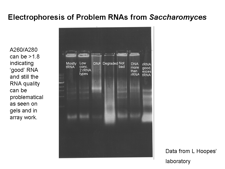
Sept 15, lab 3.  LH calls on two students to review the purpose of the experiment and what was done last week.  Quality control tests on the RNA prepared.  Students will dilute a tiny sample of their RNA and will also apply another tiny sample of it to an agarose gel for quality control.  During dye coupling, practice filtering and clustering data using GeneSpring and the cell cycle data set. Final discussion of background papers on topic of experiment and microarrays. At the end of the period, each pair of students should show the quality control data to Dr. Hoopes and discuss with her whether to go ahead with hybridization or to prepare a new RNA sample next week.

Sept 22, lab 4.  LH calls on two students to review the purpose of the experiment and what has been done so far.  LH describes briefly the Reverse Transcriptase cDNA probe synthesis protocol, cDNA purification, and hybridization for today.  Synthesis of cDNA and hybridization setup.  During the two hour  RNA to cDNA incubation today, we will meet as a class and discuss further aspects of the project chosen.  During this laboratory, students will practice gridding spots from last year's data using GenePix and Magic Spot and will practice choosing data for analysis using the cell cycle data in GeneSpring.  Write up new thoughts about hypotheses about microarray results.  Then cDNA will be purified and hybridization to arrays will be set up to run overnight. Between laboratories: TOMORROW morning at 8 or at 9, arrays will be washed to free them of unincorporated dyes.  If possible, plan to have one of each lab group pair help with the array washing/drying and scanning.  

Sept 29, lab 5. LH calls on two students to review the purpose of the experiment and progress. Students and LH describe and discuss scanning process and the type of data generated.  Class moves to SS5 at scheduled times (two lab groups can grid at once) and proceeds to grid data with GenePix.  After 1 hour, gridding work must be saved and continued at another time between laboratories, as a new set of groups will be incoming.   

Oct 6, lab 6.  Lab books turned in for grading at the end of the period.  During this lab period we will begin the more sophisticated level of data analysis from the microarrays.  Each group should have obtained an Excel spreadsheet of the GPR files, imported them into GeneSpring and filtered the data by the end of the period.  This work will continue next week in laboratory.  Between laboratoryies and in these two laboratories, each group needs to have clustered your data using hierarchical clustering (treeview) and  qCLUSTER methods.  You need to record the results of each clustering in a file, and take notes in your lab book of apparent functions represented in the genes seen in each of the clusters.     

Oct 13, lab 7.   LH will call on two students to summarize the microarray experiment so far.  Lab books will be returned;  continue the data analysis using GeneSpring  and design second array experiments.  LH will note during the grading process what kind of genes might be included in each cluster, so you can then return to your data files indicated as interesting by LH and get information on all the genes in them using SGD to get the names and functions of the gene products, or annotations.  This information needs to be recorded in your lab books, with any thoughts you have about what each clustering method has done.  In your notebook, comment on how the results compare with your hypotheses at different points.  Introduction to MAGICTool data analysis program, using the entire class data set of gene expression ratios.  In this laboratory  we will design the second microarray experiment, capitalizing on the results of the first.  Some students will use arrays again, with dye flips or other kinds of experiments, while others may choose to perform qRT PCR analysis on two genes chosen from the first data set.  For those choosing qPCR, primers must be designed and ordered this week.  Discuss with LH the quality control you will be doing next week after fall break.

Oct 20, lab 8:  Begin the second microarray or qPCR laboratory work.  Students prepare and present material about the technique of  quantitative Reverse Transcription PCR.    The students using microarrays for a second experiment will plan collection of the samples for the RNA preparations needed.    If doing qPCR, you need to do quality control DNA PCRs today to make sure the primers you designed amplify the right size of fragment and run a gel on them.  Depending upon the number of groups doing  qPCR, we may run one or two gels.  Make sure to show on the gel diagram where your sample is loaded as well as the gene being tested and the predicted size of the product..  The rest of the time today can be used to follow up on your data analysis from the microarrays.  Also, each group needs to sign up for data analysis periods next week in SS5, for the class microarray data already collected.

Oct 27, lab 9.  LH will be away at HHMI program director's meeting Oct 25-Oct 28 so  laboratory will be informal and will consist of continuing cluster analyses of your data using GeneSpring and MAGIC Tool at times during the week that are convenient for the student groups.  Make sure to note in your lab notebooks when you worked and on what you worked, as well as notes on the results. 

Between laboratories:  Between laboratories the cells should be grown and harvested and snap frozen for future RNA preparations, according to your approved plans for the next experiment, before the next laboratory period.  Also, if doing qPCR, you should redo quality control PCR and/or redesign primers and order new ones if needed; consult with LH and Laty.

Nov 3. lab 10. Preparation of new RNA samples for arrays or qPCR. Using the same method as in the earlier laboratory on RNA preparation, today you will prepare RNA from your samples of cells you grown and  frozen and also today you will run the quality control gels and get absorbance ratios for second RNA preparation for array analysis or qPCR.   Consult with LH to make sure the RNA quality is acceptable.

Nov 10, lab 11.  cDNA labeling and hybridization of second set of microarrays or setup of qPCR.  We will discuss and review the method before we begin, if possible, one of each lab group doing arrays needs to attend and help with the washing and scanning of the arrays.   If doing qPCR, we will collect the data from all experiments in the morning.   Two computers in SS5 have the software for the ABI Prism 7000 on them and can be used for studying the data.  You should also copy the data from the table at the end of the output into Excel so you can calculate the ratio of expression to our control gene, TUB1.  If doing microarrays, you will need to grid your data during this week or next week.  Signups for data analysis periods will be scheduled during lab, so bring your calendars!

Nov 17, lab 12.   Microarray data sets for each array (Tiff picture files at two different wavelengths) will be put onto CDs and made available for pickup in the laboratory or LH's office.  Students need to grid and collect data and give the normalized GPR files to LH for posting in the class data space on the H server by the end of Monday, Nov 22.  Sign up for data analysis time the weeks of Thanksgiving and Nov29-Dec3 TODAY in lab; bring calendars!

Nov 24,  lab 13.  Makeup/data analysis laboratory.  If you have fallen behind due to RNA quality control or otherwise need to do wet lab work, this day can be used for it.  It's the day before Thanksgiving, so lab is optional.  If you've signed up for time to work on data analysis in SS5 during this lab, it will relieve the crunch next week.

Dec 1, lab 14, Data analysis/ work on report on class project.  Using the data posted for microarrays and the qPCR data collected by others in the class, complete the data analysis using GeneSpring, MAGICTool, and ABIPrism7000 software plus Excel for the class project.   Data analysis using GeneSpring in the computer laboratory.  Import all of the class microarray data from both sets into GeneSpring and complete the filtering and clustering.  Make notes on how you filtered and clustered (what your settings were and which cluster method you selected) and what you found out.  Save clusters and gene lists; use PIR gene lists to find out what kinds of processes have changed in your tested cells.  Save plots and print a few for your report. OR use MAGICTool and make a correlation matrix and cluster using the various clustering options in that program.  Also, make sure you have analyzed the data from the quantitative PCR experiments done, and related those to the results from the microarray experiments.  Write up notes on when/on what you worked in lab notebook, and write up a short paper on the findings of the class analysis.  Paper should be 3-4 pages plus graphs, charts, calculations should be shown in detail.   Papers are to be individual efforts, although discussion during analysis is encouraged.    Log into the GCAT site and take the post-microarray survey there.

Dec 8, Last laboratory,  wrap up session: students must attend and participate in final discussion; laboratory books and the short paper on the class project due; all materials must be turned in to instructor and all unwanted materials discarded appropriately during this period.  

2004 Experiment

GenReg Laboratory Group Project Choices for 2004.

Constraints on everyone:

We will only do ONE group experiment in the class, in order to get what we hope will be a significant amount of data addressing our class question.  Each lab group (two students) will be able to do ONE microarray slide in the first round of experiments.  In the second round, about half of the lab groups can work on one more microarray and about half can work on testing the expression of genes identified from the microarray experiments by means of real time reverse transcriptase PCR experiments.  So, plan your tests/controls so that 6 microarrays, with perhaps 3 more to test vital points or provide replication, will be enough to address your questions/hypotheses.

1.  Nucleotide Excision Repair Gene Expression  

    Background:

Yeast, like most eukaryotic cells, has multiple DNA repair processes.  One of the most important in all kinds of cells is nucleotide excision repair, NER.  In yeast, a complex of two proteins, Rad1p/Rad10p, is a vital part of the NER pathway that makes incisions near a site of DNA damage such as a thymine dimer or other bulky adduct.  Without either of these two proteins, i.e. in strains deleted for either of the two genes encoding the dimer, there is greatly increased sensitivity to UV damage (killing). 

1.  Paper shows that just a few genes are induced by DNA damage, regardless of the type of damage (but not including UV damage or looking at a mutant affecting NER):  Gasch, Audrey P. et al, Genomic Expression Responses to DNA-damaging agents and the regulatory role of the yeast ATR homolog Mec1p.  Mol Biol of the Cell 12:2987-3003(2001). 

2.  Prakash, S and Prakash, L.  Nucleotide excision repair in yeast.  Mutation Research 451:13-24 (2000).  Paper reviews the role of various enzymes in NER process, and shows that complexes exist with the NER proteins associated with other pathway proteins, especially those needed for transcription with RNA polymerase II (TFIIH is a protein that stimulates RNA pol II transcription).  Review article providing background and perhaps ideas about what genes might be affected in NER mutants.  

Strains available: Wild type W303a; T177, a W303a strain in which rad10 has been deleted and which is therefore deficient in nucleotide excision repair and sensitive to UV irradiation. 

 Other information and resources: 

1. Last year’s class tested T177 compared to wild type without UV treatment and found little or no difference in mRNAs assessed via microarrays; this data set is available to be compared with any new data.  Other available data in our lab include microarray data from  wild type/wild type comparisons, rad52delete/wild type comparisons (2 available on our computers).

2.  We have a Stratalinker which can be used to provide UV irradiation to cells on plates.  Cells in liquid don’t receive UV very well, since the water base of the liquid medium absorbs most of the UV energy.

3. UV damage can be repaired by a photoreactivation system that will reverse the damage; in order to prevent photoreactivation from acting to reverse the DNA damage to which you want the cells to respond, you can wrap the container(s) of UV irradiated plates or tubes with aluminum foil to keep out visible light.

4.  Attached is a survival curve for wild type and for T177 yeast prepared by Adam Simning for his senior thesis; it may be helpful in designing experiments.

2.     Energy metabolism in petite strains from yeast.

Background: 

In yeast, if wild type cells are grown on rich medium with ethidium bromide added to it, they tend to lose all or part of their mitochondrial DNA and become respiratory deficient cells that make small colonies (‘petites’, also known as rho minus or r-).  This characteristic is inherited by the progeny cells even when propagated without the ethidium bromide medium.  Since the mitochondrial genome encodes important subunits for some of the electron transport carriers, the electron transport and oxidative phosphorylation reactions cannot occur; the petite cells must grow by fermentation and can grow without oxygen by fermenting glucose to form ethanol. 

Paper 1: Epstein, C. B. et al., Genome-wide responses to mitochondrial dysfunction.  Mol Biol of the Cell 12:297-308 (2001).  Paper shows microarrays of petites and wild types; of course, every time a new petite strain is isolated, there is a chance that a different part of the mitochondrial genome is deleted so there may be differences between his petites and any we isolate here in terms of their gene expression data.  The study suggested an induction of peroxysomes and interaction with the retrograde regulatory genes that participate in mitochondrial/nuclear cross talk in petite strains.  A few different inhibitors and media that would allow only anaerobic or only aerobic growth were tested in this paper; others would be interesting.  For example, what about adding malonate, a competitive inhibitor of an enzyme of the Krebs Cycle, Succinate DeHydrogenase?  What might that do to gene expression in a petite versus wild type? 

Paper 2: (Not in packet, just for you to know about!) Taylor, D et al.  Conflicting levels of selection in the accumulation of mitochondrial defects in Saccharomyces cerevisiae.  Proc Natl Acad Sci, USA 99:3690-3694 (2002).  Paper cites human degenerative diseases that result from mitochondrial genomic changes, and analyzes mathematically a situation in which defective mitochondria should come to predominate (within- and among-cell selection values were manipulated by the modeling team).  This one is so you will realize the weird ‘petites’ of yeast have potential to help us understand human diseases!

Paper 3: DeRisi, J, Iyer, V and Brown, PO.  Exploring the metabolic and genetic control of gene expression on a genomic scale.  Science 278:680-686 (1997).  Looks at diauxie, which Paper 1 compares with the petite gene expression patterns.

Strains available: W303a wild type, and some strains selected for small colonies on several rounds of ethidium bromide-containing-YPD medium so they presumptively are petites.

 Experiment chosen:

Nucleotide Excision Repair in Deletion

Design of Nucleotide Excision Repair Experiment, 2004; concepts prepared by NER team with LH following their guidelines...

 Both the W303Ra wild type (YLH208 stock) and the T177 deletion of RAD10 (YLH268 stock) were streaked out on YPD medium and single colonies grown.  A well isolated colony was used to inoculate 5 ml YPD liquid medium which was incubated overnight with shaking.  At 10 AM, larger culture flasks of YPD were inoculated with 1 ml/100 ml medium from the overnight stock culture.  For the wild type, 150 ml was used; for the T177 200 ml was used (since it sometimes grows a bit more slowly).   These cultures were grown with shaking until 3:30 PM. Cells were spun out in sterile 50 ml tubes and the media discarded.  The cells from each of the two strains were resuspended in about 3 ml PBS and distributed equally into 6 sterile microfuge tubes.  The tubes were spun 2.5 minutes at 10K x G and the supernatants discarded.  Each was thoroughly resuspended in 100 ul PBS. 

For each strain, 3 tubes of cells, meant to serve as the control samples for the three microarrays from that strain, remained at room temperature in the PBS.  The remaining three samples were transferred to a YPD agar plate and irradiated with a dose that is predicted to produce 75% viability when photoreactivation is not permitted (where we expect very good repair, as opposed to lots of cell death with heavier doses).  For wild type (208) this dose was 25 Joules/meter squared while for the T177 (268) it was 2 Joules/meter squared.  Two of the three plates were wrapped with foil immediately after irradiation.  All three were incubated at 30 degrees. 

One foil wrapped plate’s cells were collected from the agar surface after 5 minutes of recovery, using foil to keep light exposure to a minimum.  To collect the cells, 0.7 ml of PBS was micropipetted onto the plate, the surface was swept with a sterile glass spreader, and the suspension was sucked up into a P1000 micropipettor.  This procedure was repeated to increase yield of cells.  The 5 minute sample and all three controls were then spun out and the supernatant liquid discarded; the cell pellets were frozen at -20 degrees.  After 15 minutes at 30 degrees, the cells from the other foil wrapped plate and the plate without foil were resuspended, collected, and frozen as described for the 5 minute plate, keeping light exposure to a minimum for the plate kept under foil during incubation.  Therefore, we have the following sets of samples for RNA preparation for use on microarrays.

          Control sample:                                Irradiated sample:

Array 1:  Wild type (208)                           (208) UV, 5 minutes recovery, foil

Array 2:   Wild type (208)                (208) UV, 15 min recovery, no foil

Array 3: Wild type (208)                            (208) UV, 15 min recovery, foil

Array 4: T177 (268)                         (268) UV, 5 min recovery, foil

Array 5: T177 (268)                         (268) UV, 15 min recovery, no foil

Array 6: T177 (268)                         (268) UV, 15 min recovery, foil

Protocols provided:

Microarray protocol 1: Preparation of total RNA from budding yeast frozen cell pellets.

Microarray protocol 2: Quality control tests of total RNA of yeast.

Microarray protocol 3: ISB method for direct labeling of cDNA with CyDyes.

Microarray protocol 4: Hybridization and washing of arrays.

Microarray protocol 5: Scanning, gridding, and intensity collection from microarrays with GenePix.

Microarray protocol 6: Analyzing data with GeneSpring and MagicTool.

Microarrays, Protocol 1:

Preparation of total RNA from yeast with Qiagen RNeasy kit. (Notes based on Michelle Wu protocol/LH lab)

Materials

Qiagen RNeasy Mini kit #74104

Qiagen DNase I kit #79254

Sigma Acid washed glass beads #G-8772

Sigma b-mercapto-ethanol #M6250

Special notes on procedures:

Use a maximum of 2.5´10⁸ cells per column.

The glass beads may stick to the outside of the screw cap tube along the ridges, preventing a proper seal of the tubes during breaking of the cells.  Try NOT to get beads on this area.  If you do, consult the instructor.

Add 10 ml b-mercapto-ethanol per 1 ml RLT buffer in the kit (stable for 1 month after addition of b-ME).

After disruption, all steps of the protocol should be performed at room temperature.  Work quickly through the procedures. Also do not let the centrifuge cool below 20ºC.

Each aliquot of DNase I is 21 ml and stored in the microarray box in the -20ºC freezer.  Add 140 ml buffer RDD, stored at 4 ºC, for 2 sample digestion.

USE RNA PARANOIA THROUGHOUT PROCEDURE!!  Gloves, RNase Erase all benches, do not open tubes with bare hands, try to only handle tubes through gloves to keep RNase fingerprints as far away as possible.

 Glass bead grinding of cells.

1. Wash the cell pellet with PBS (Add 200 ul of PBS, vortex, spin 2 min top speed in microfuge, discard PBS).
2. Add approximately 600 ml of acid-washed glass beads to a tube that fits the bead mill (2 ml conical, screw cap tubes).  Be careful not to get beads in the threads of the screw cap.
3. Resuspend the cell pellet with 600 ml Buffer RLT + b-ME.
4. Add the resuspended cell to the tube with glass beads.
5. Use setting 3, 50´100 rpm, and 30 second each session on the Biospec Mini-Bead Beater.  Wait for a substantial number of the 8 tubes it holds to be loaded before you begin the shaking.
6. After each 30 seconds session of vortexing on the homogenizer, chill the tube in a ice+ water bath for at least 30 seconds.  Repeat homogenization 6 times total.
7. Transfer lysate to a new 1.5 ml tube and centrifuge at top speed for 2 min.
8. Transfer the supernatant to a new 1.5 ml tube and measure the volume with 1 ml pipettor (~350 ml)  NOTE: to measure the volume with the P1000, set the dial BELOW where you think the volume will be, for example at 250 ul.  Take up the volume, and there will be some liquid left in the tube.  Keeping the tip in the liquid, dial the volume setting up until you have just taken up the last of the liquid but no air.  Record volume.  Strive NOT to introduce a lot of air bubbles, for example don't pipet up and down repeatedly or suck up a lot of air.
9. Add equal volume (that is, 350 ul or whatever you just measured the volume to be) of 70% ethanol and mix gently by pipetting.
10. Load the sample to a RNeasy column including any precipitations.  Each column has a max loading volume of 700 ml, load with first 700 ul and then load with rest of volume if the volume exceeds 700 ml.
11. Centrifuge the column for 15 sec at 10,000 rpm. (Share the centrifuge!)
12. Pipet up and discard flow through in the b-ME waste tube.
13. Wash the column with 350ml RW1 buffer, and centrifuge for 15 sec at 10,000 rpm.  Pipet up and discard the flow through.

 DNase Digestion

14.  Add 140 ml buffer RDD to the 21 ml aliquot of DNase I.  Gently pipet to mix.  DNase is especially sensitive to physical denaturation, mix gently, do NOT vortex.

14. Pipet 80 ml the DNase to the center of the membrane without touching the tip to the membrane, and incubate at room temperature for 30 min.  Digestion will be incomplete if DNase I sticks to the walls or the O-ring of the column.
15. Wash the column with 350ml RW1 buffer, and centrifuge for 15 sec at 10,000 rpm.  Pipet up from the bottom tube and discard the flow through.
16. Wash the column with 500 ml RPE buffer.  Centrifuge for 15 sec at 10,000 rpm.  Pipet up and discard the flow through.
17. Repeat step 17.
18. Transfer the column to a new, supplied 2 ml collection tube, centrifuge max speed for 1 min to dry the membrane and eliminate any residual RPE (which interferes with elution).
19. Transfer the column to a supplied 1.5 ml tube.  Pipet 30 ml RNase-free water directly to the center of the membrane without touching and incubate for 1 min.
20. Centrifuge to elute, at 10,000 rpm, 1 min.
21. Repeat the elution again, total elution volume ~ 60 ml.

Total RNA absorbance measurements.

23. Turn on the UV lamp from the spectrophotometer to wavelength 260nm.  Allow 15 min warm up time.
24. Take a tiny sample (2 ul); dilute sample 1:200 with MQ H₂O, to total of 400 ml.  Take a second
25. Use the quartz cuvette for absorbance reading. 
26. Rinse the cuvette with MQ H₂O several times and zero with no less than 400 ml.
27. Read the absorbance of the sample at both 260 nanometers and 280 nanometers, and calculate the amount of total RNA: A260 reading ´ 37mg/A260 reading ´ dilution factor = total mg RNA / ml sample.  NOTE: the Dilution Factor is the amount you have diluted the sample before taking its absorbance.  In this example, you have diluted it 200 fold, so your dilution factor is 200.   Also, calculate the A 260/A 280.  For acceptably purified RNAs, this ratio is expected to range from 1.8 to 2.2.  We may use RNA with a lesser ratio, depending upon the appearance of the gel.
28. Clean the cuvette with several changes of MQ H₂O.
29. Remove a sample of 3 ul of each of your RNAs to a clearly labeled tube that you will hold on ice until needed, for use in a quality control gel electrophoresis (see below).
30. Your sample now has nominal volume of 60-5 ul or 55 ul.  To precipitate it for use in the next procedure, add 0.1 volume (5.5 ul) of 3M sodium acetate, pH 5.2 and 2 volumes (121 ul) of 100% ice cold ethanol.  Mix by vortexing. Place on dry ice powder for at least 5 minutes.  Spin in refrigerated microfuge 5 minutes at top speed.  Use a pipettor to remove all liquid.  Cover the top with parafilm and, using a sterile instrument, poke about 5-6 holes through the film.  Place tube at 37 degrees for 10 minutes.  Make sure it's labeled clearly with your names, type of sample, date.  With gloved hands place in Bio 164 box in -20ºC freezer until next lab. 
31. To each of your electrophoresis samples, add 1 ul of gel loader dye mix and 2 ul of RNase free water.  We will use an 0.7% agarose gel in 0.5x TrisBorateEDTA (or TBE) buffer with ethidium bromide stain (a possible carcinogen, so do not get touch the gel or buffer); the gel has been prepared  for you to use.  Spin the two electrophoresis samples briefly to get the entire samples to the bottoms of the tubes.    Also make a drawing of the gel in your lab notebook.  The instructor will keep the map in her notebook for future reference.  Each gel holds a maximum of 8 samples, and one lane will be used for a standard.  When 4-6 lanes are loaded, tell the instructor, who will  load the standard into one of the slots.  The standard will be provided with tracking dye already in it.  When the samples and the standard are loaded, we will begin the run at 75 volts and continue it for 1 hour.  The gel contains dye, so it is ready to examine at the end of the hour.  Wear gloves and goggles, and photograph at the gel.   At the end of the lab, each person should have an image of the RNA quality control gel(s) containing your samples for his/her lab notebook.  Refer to the image below to assess the quality of your own and the other groups' RNA samples.  Be sure to comment in your notebook about the quality of the RNA (your own, and the other samples on the same gel as well). After these quality controls are complete, Dr. Hoopes will decide whether each RNA is suitable for arrays.  If not, we will need to prepare a second batch of RNA to use.

 Microarrays, Protocol 3:

Direct Incorporation of Cy3/Cy5 During Reverse Transcription(Method from Institute for Systems Biology, 2003, with notes by Todd Eckdahl and Anne Rosenwald)

Materials Needed:

Isolated and quantitated total RNA samples

Microarray slides (70-mer plus-strand oligomers)

RNase-free water

oligo dT primer (16- to 18-mer) at 1 mg/ul

Coverslips, 22 x 40mm size from Corning

100 mM DTT (dithiothreitol)

low dTTP dNTP mix (10 mM each dATP, DCTP, dGTP, 1 mM dTTP)

Cy3-dUTP and Cy5-dUTP (1 mM each [separately])

3 M Ammonium Acetate, pH 5.2 (OR 3M Sodium Acetate, pH5.2)

100% Ethanol, 70% Ethanol

Enzymes:

Superscript II Reverse Transcriptase, 5X first strand buffer

RNase A (4 mg/ml)

RNase H (2 unit/ml)

Reverse Transcription and Cy-dye Incorporation

1. Prepare two tubes containing the two different RNA preparations you wish to compare via microarrays as follows: obtain a dried aliquot of 50 mg total RNA (one for each treatment).  This RNA must have been:
   1. already checked with denaturing agarose gel
   2. quantitated with UV spectrophotometer (and A260/A280 obtained)
   3. precipitated (eg. 1/10 volume 3M NaOAc pH 5.2, 2 volumes EtOH) (Note: These instructions will be given at the end of the RNA prep laboratory; however, if you were given the RNA in solution, for a 30 ul sample you would add 3 ul of the salt such as sodium or ammonium acetate and 66 ul of 100 % ethanol, cold.  Mix by finger vortexing.  This solution should be brought to freezer temperatures before centrifugation either by sitting in -20 degree freezer for 20-30 minutes, sitting in powdered dry ice for 3 minutes, or being flash frozen in liquid nitrogen.  Now spin at top speed for 5 minutes in a microfuge, ideally a chilled microfuge.  Remove the supernatant using a pipettor and tip, not by decanting/dumping out.  Get out and discard every visible bit of liquid.  Allow the pellet, which may or may not be easily visible, to dry as follows.  Cover the open top of the tube with a piece of parafilm and poke 5-6 small holes through the file.  Allow tube to sit for 10 minutes with the top open at 37 degrees.  Sniff to see if any ethanol odor remains; if it does, let sit longer at 37.)
2. To each tube of dried RNA, add 2.5 mg oligo dT
3. Add 8.5 ul of DEPC-treated H₂O and gently mix, for a total of 11 ul.
4. Heat to 75^oC for 10 min in a PCR machine or temp blok.
5. Cool slowly to room temperature and spin down (Note:  keep at RT from this point on)
6. Add the following in order:
   1. 4 ml Superscript first strand 5X buffer
   2. 2 ml DTT (100 mM)
   3. 1 ml dNTPs (10 mM each dATP, dCTP, cGTP and 1 mM dTTP)
   4. 1 ml Cy-dye labeled dUTP (1 mM) (One gets Cy-3 dUTP and one gets Cy-5 dUTP)
   5. 1 ml Superscript Reverse Transcriptase II (200 units/ ul; make sure this is Exonuclease-free)
7. Mix gently and incubate at room temperature for 10 min
8. Incubate at 42^oC for 2-3 hours (no more than ~5 hours; do not do this step overnight)
9. Heat sample to 95^oC for 2 min
10. Place samples on ice, spin down (can store at –20^oC at this point if necessary)

 Degrade RNA

1. Make sure contents of tubes are spun down
2. Add 0.5 ml of RNase A (4 mg/ml) at room temperature (Promega)
3. Add  0.5 ml of RNase H (2 U/ml) (Fermentas) (Note:  Not clear if really necessary to use both enzymes; the RNase H is fairly expensive)
4. Incubate at 37^oC for 15-30 min

 Purification (Using Qiagen PCR CleanUp Kit)

1. Add 25 ml high-quality H₂O to samples , mix gently.
2. Add 2.7 ml  3 M Sodium Acetate, pH 5.2, mix gently.
3. Add 250 ml QIAquick  buffer PB, mix gently.
4. Apply each sample to a QIAquick column (the DNA should stick to the column here)
5. Centrifuge for 30 sec at full speed
6. Take the column flow-through and replace back onto the top of the column and spin a 2^nd time
7. Place the flow-through back in the original tube and save in case of problems with the purification.     
8. Wash with 400 ml QIAquick buffer PE, spin 30 sec at full speed and discard flow-through (your DNA remains on the column)
9. Repeat step 8, discarding flow-through
10.  Spin the column briefly once more to get rid of remainder of wash solution
11. Place column in a clean, well-labeled 1.5 ml elution tube
12. Apply 30 ml DNase-free and RNase-free water to center of column without touching the membrane
13. Wait one min, then centrifuge 1 min at full speed (gradually increase from 0 to full speed to avoid shearing off the Eppendorf tube lids).  Your cDNA is in the flow-through this time!
14.  Reapply THE SAME 30 ml water to center of column without touching the membrane.  Wait 1 minute, spin, collect eluate.  Now the doubly eluted cDNA should be in a volume of ~30 ml for each of your two samples.
15.  Continue from the hybridization protocol.

Microarray Protocol 4: Hybridization and Washing of Microarrays.

 (Based on notes of Todd Eckdahl from procedures of Institute for Systems Biology, 8/03)

Microarray Slide Processing

This procedure is optional for oligo slides (Isb or WU slides); it redistributes the oligo DNA on the slides, which helps spot morphology and hybridization.  It is mandatory for PCR product slides (TMC or Stanford slides) , otherwise the duplex DNA will not be opened up for hybridization.   Some PCR product slides may not have had earlier steps in post printing processing done and may need additional steps; check with the array providers to be sure.

     1.      Steam the DNA side of the slide over boiling dH2O.  Do not allow visible droplets to form on the slide.

2.      Immediately place the slide (DNA side up ) on a heat block or hot plate set to 100 C or slightly less to snap dry.  Take off after 5 seconds.

3.      Repeat steam step, followed by drying step.  Allow the slide to sit on the heat block for 15 seconds this time.  Allow slide to cool.

 Prehybridization and Blocking

        1.      Place slide into a 50 ml tube filled with warm (55 C) 3x SSC, 0.1% SDS, 0.1 mg/ml Sonicated Salmon DNA. 

            The slide must be completely immersed. 

     2.      Agitate gently for 30-60 minutes at room temp. by rocking on a platform (lay the tube down flat on the rocker but

            wedge it so it will not roll off).

3.      Quickly transfer the slide to a 50 ml tube with dH2O.  Dip several times.

4.      Blow the slide dry with air or spin it 5 mintues in a clinical centrifuge in a dry 50 ml tube.  If blowing dry, the idea is to chase all the drops of water off the slide while it is held at an angle on a towel.  If drops of water start to dry in place on the array, quickly immerse the slide back into water and start again. You are not trying to blow dry the slide, rather you are trying to push the liquid away from the spots. If you see streaks at this stage, rewet the slide. If you see dried-on streaks, you will have streaks in your final scan.

 Labeled Sample Preparation and Hybridization

         1.      Combine 30 ul (entire sample)  of each cDNA with its dye into a single tube and Speed-vac to 1-2 ul.  If

                sample dries (avoid this if possible!!), add 2 ul DEPC-H2O and let stand 2 minutes (slight warming is OK).

2. Add 40 ul of the following Hybridization Buffer
   1. 36.4 ul DIG Easy Hyb
   2. 1.8 ul of 10 mg/ml denatured salmon sperm DNA (or calf thymus DNA)
   3. 1.8 ul of 10 mg/ml yeast tRNA (optional: replace with 1.8 ul of DIG Easy Hyb)
   4. 0.14 ul of 1 ug/ul oligo dA (ideally 50 dA's long, but shorter ones also work)
3. Mix the sample gently to distribute the two dyed cDNAs throughout and heat at 90 C for 1 minute (in a temp blok or PCR machine). 
4. Place on ice 1 minute.
5. Heat at 90 C for 5 seconds, then spin down.  Keep in the dark under foil until used.
6. Blow dust off microarray slide using Whoosh Duster spray can if necessary.
7. Prepare cover slip by dipping in 100% isopropanol and blot with lens paper (or in a pinch, Kim Wipes). You don't want to polish the coverslip as that would develop an electric charge on it; just blot it dry a few times.
8. Load the array with the cDNAs in Hyb Buffer.  Choose, and ideally practice with a blank slide, one of the two loading methods presented below.   Method A.  Pipette sample onto one end of the array.  Place one end of the cover slip onto the end with the sample.  Use a fine gauge syringe needle to lower the other end (between 70% and 95% of the spots should be wetted) of the cover slip but raise it back up before the solution makes its way over the entire area.  This serves to mix the sample while it is applied to the array.  Then let it down all the way, withdrawing the syringe needle.  Method B.  Place the entire hyb buffer and cDNA sample on the cover slip.  Invert the array slide and use it to pick up the coverslip, inverting the paired slide and coverslip before the liquid has spread out to the sides of the slide. 
9. Place the slide in a hybridization chamber.  Load 10 ul of sterile water into each of the two little wells at the ends of the chamber.  Seal up using the top and the black slider clips and incubate at 37 C for 15-16 hours.

Posthybridization Washing

1.      Heat 50 ml 1X SSC / 0.1% SDS and 0.5X SSC to 55 C.

2. Transfer slide to heated 1X SSC / 0.1% SDS  using forceps that touch ONLY the Label NOT the spotted area.  Place slide with cover slip facing down and agitate gently until coverslip falls away from the slide. Using the forceps, pull up the slide just enough to make sure the coverslip is completely detached from the slide and resubmerge the slide.   Remove the cover slip with the forceps and discard it.  Agitate the slide gently (laid flat on a rocker) for 5 minutes under foil.
3. Dump wash solution and fill immediately with fresh 1X SSC / 0.1% SDS at room temperature.  Agitate gently for 5 minutes under foil. Do not let the slide dry at all.
4. Dump wash solution and fill tube with 55 C 0.5X SSC.  Agitate gently for 5 minutes under foil, inverting the tube a couple of times. Do not let the slide dry at all.
5. Dump wash solution and fill tube with 0.1X SSC at room temperature.  Agitate gently for 2 minutes under foil, inverting the tube a couple of times. If you are going to have to wait for the centrifuge in step 7, keep the slide in this solution until just before you can spin it dry.  Do not let the slide dry at all.
6. Transfer slide quickly to a 50 ml tube with dH2O.  It can only stay in this solution a couple of seconds before all of the fluorescent cDNA will come off, so DO NOT store it in this solution while waiting for the centrifuge.  Instead, stop in the step 5 solution, dip in the water just before you are going to spin dry.
7. Centrifuge in a dry 50 ml tube for 5 minutes.
8. Keep dry and in the dark until scanning. 

 Microarray Protocol 5: Scanning, gridding, and data collection

Scanning on AxonGenepix scanner.

We use our Axon GenePix 4000B scanner, currently located in SS5, to scan the microarrays.  For more information about the material below, you can refer to the help tab in the GenePix Pro software for more about any item given in italics.

1. Turn on the scanner; check to see if the correct dongle is installed in the ISB port of the computer running the 4000B and then start up the GenePix Pro 5.1 software. 
2. Slide the scanner door open.  Holding the microarray so that you do not touch the spots, insert the array with the label end towards you and the hybridization side DOWN.  (NB  If you are not sure which side of the array has the spots/hybridization, you may breathe gently onto the array through your mouth; if the array side is ‘up’ the spots will become visible for an instant or two).  Clip the chip holder easily around the slide.  Do not push directly down onto the clip.
3. Using the software on the computer, use the ‘Hardware settings’ (upper left of screen) window to set the Photo multiplier tubes (PMTs) both to 600, for the 635 nm (Cy5) and the 532 nm(Cy3) channels.  This is a first approximation; they will need to be reset later on.
4. Perform a low resolution “Preview Scan” to determine the location of spots and the initial hybridization intensities.
5. Using this scan, if you are able to locate the entire region where the spots occur you can draw a marquis around the entire array of spots, leaving out the blank areas so they will not take up pixels in your data scan file.  To do this, choose “Scan Area” and click and drag to draw in the rectangle around the array spots.  If you are not sure you are seeing all of the spots, you may need to adjust the PMT settings and repeat the Preview Scan to find the spot area.
6. Make another guess as to best settings for the PMTs, for example if red is high and green is low, increase the green or decrease the red by 50. 
7. For gene expression hybridizations, we will eventually attempt to make the ratio over the entire scan area as close as possible to 1.0.  You will raise/lower the two PMTs to achieve this color balance more stringently later on.
8. Before you collect data, change the ‘Lines to average’ in the ‘Hardware settings’ to 2.  The scanner will now scan each pixel twice and average the two, reducing any background noise that may be present.
9. Adjust PMTs for the two colors carefully based on histograms, as follows.  Start up a high resolution “Data Scan”.  As the image is scanning, go to the “Histogram” tab located at the top of the screen.  The histogram that appears, color coded red (Cy5) and green(Cy3), allows you to observe the relative intensities of both channels as you scan.   Settings for the histogram should be:            Image: Both

                                                                    X axis: Fullscale

                                                                    Y axis: Log Axis on Fullscale

The histogram that appears shows you the percentage of Normalized Counts that are at a given Intensity.  Note that the histogram only shows you the pixels that you are viewing in the image tab; i.e., if you are zoomed in on the image, it will only show the zoomed in area in the histogram.  Remember that every pixel is represented in the histogram, so artifacts and dirt will skew the readings.  If you have a lot of artifacts or dirt, try to zoom in on a clean portion of the array to determine more appropriate PMT settings.  You can avoid the dirt later in the gridding process.  Adjust the two PMTs during this ongoing data scan so that you can see similar histograms of pixels across the entire intensity range.  Note, though, that saturated pixels (with counts greater than ~67,000) will be thrown out and spots with pixel counts close to background will result in poor data, so you don’t want to ‘correct out’ all of your intensity in either channel.

10.   Observe the Intensity Ratio; when it is approximately 1.0 then perform a totally new ‘Data Scan’ over the ‘Scan Area’.
11.  Save the scan results even if you think it does not look useful; it might be used for a different purpose and arrays are too expensive to run to simply throw out the data!!  To save, go to the ‘Open/Save’ button and select ‘Save Images’.  Save the images into the Bio164 file on the Desktop.  Select as the image type = Multi-image Tiff Files.  Do not save the preview or Export Images, instead only save the wavelength 635 and wavelength 532 images.  Name the files including a date prefix and indicating the type of experiment.  (Example 1: 031904_1.5Gchlor_dyeflip  indicating a study done on March 19, 2004 of 1.5 Generation cells grown with Chloramphenicol, with the Cy3 and Cy5 dyes flipped from the ‘usual’ symmetry of Cy5 on the experimental sample and Cy3 on the control.  Example 2: 101003_b164SP_rad52del_635, indicating an experiment done October 10, 2003 by Supriya Patel in Bio 164 using a deletion of rad52, this file being the 635 nm data from that experiment).  Note that to continue collecting data from an experiment, this program is saving a greyscale image of each channel's color.  The program will overlayer them and use false coloring to make the 635 look red and the 532 look green; if both are present it will look yellow.  If you fail to save these two files, there is no way to quantitate your data.
12. Once your images are successfully saved you are ready to assign spot identities and calculate results.  We have taken the gene lists for our array slides, giving the number of tips used to print, positions of each oligo in the 384 well plates used as a source for the DNA printed, number of 384 well plates used, and spacing between spots, and converted them into GAL files (Genepix Array List) using the program.  A copy of each GAL file you might need is stored in the Bio164_04 folder on the Desktop.  We have also stored a copy of a .gps file for each of these GAL files.  The .gps file is a set of stored grids with spot indentities; the grids may not position correctly at first, but you will be able to optimize their placement. Continue now or at a later time by creating and positioning grids as described in the following protocol.

GenePix 5.0 Spot Finding

Preparing the image for quantitation:

1.  Open GenePix 5.0 with the dongle installed in the computer.

2. Click on the right side menu on the disc to bring up stored files; choose Open Image, then find the file you are using and select the two TIFF files (green and red) that need to be opened. (You will need to hold down the shift key when selecting the second one). 

3. Load the grid file: click on the disc icon on the right and choose Open Setting.  Then find the file you need with the gps settings for the chips we are currently using.  Double click on the desired file to load.

4. Set the left side menu to “block mode” (square with up arrow on left side).  Now, click on the Zoom key (magnifying glass).  Then you can use click at upper left and drag to desired lower right to select the part of the image with your data and the grids in it and zoom it to full screen.

Preliminary positioning of grids for automatic spot finding:

1. Click on block mode (square with left top arrow) and select all grids using mouse click and drag; then use the mouse to arrange all the grids at once so that they seem to fit all data.
2. Zoom in using the magnifying glass key.  Check that you are still in block mode. Position the upper left block in the window (using > and < keys from keyboard and/or screen arrow bars) and zoom in to make it fill the window but have all corners visible.   Make sure you are in block mode again. Click outside all grids and then click on that grid to select it alone.  You will see white dots at various locations around the selected square; make sure they are just on your selected square before proceeding.
3. Use the mouse to move and/or rotate that grid using the white dots as mouse positions until it lines up as well as possible with your colored dots.  You probably won’t have to rotate grids much if at all.  Focus on where the upper left and lower right corners are located, as the software can do the rest on its own pretty well.
4. Move on to the grid to the right and repeat positioning.  Finish that row and then move to the left grid in the next row down, etc.  Repeat until all grids are roughly positioned.
5. Zoom out (use the “undo zoom key next to the zoom key), make sure you are in block mode (square with left top arrow), and then select the whole grid.
6. Push the F5 key on the top line of the keyboard; this will find all features (spots) automatically.  Repeat the F5 command.
7. Save: choose “Save settings as” and name the settings file with the tif file name without the wavelength, e.g. Yg_rad10-Top.gps.

Refine positions of spots before collecting data.

1. Make sure you are in block mode (box with upper left arrow).  Zoom in to block number 1 and select it (upper left grid/spots).  Spots will have been resized by the F5 feature finder, and most will be correctly sized and positioned. 
2. Change to feature mode (circle with up arrow and California state to right).  Now when you mouse click on a spot, it will select it and you can move it with the mouse to center the circle on the spot.  If you need to change the size of the circle, it must be selected and then you push the Ctr key plus one of the four directional arrow keys to change the size.
3. Some of the spots are ‘flagged’, that is there is a vertical line drawn in them to tell the quantitation program that they are suspect spots.  You can add or subtract spots from this designation as follows.  To flag a spot, select it and press the “a” key on the keyboard.  To deflag a spot, either move it off the colored spot or select the spot and press the ‘l” key.  If unsure about flagging a spot, in feature mode you can double click on the spot to see the regression of one color on the other across all pixels; if it’s a ‘good’ spot, there should be one straight line.  You can look at where the background pixels are and where the feature pixels are on the regression spot by selecting each separately from the menu shown with the regression.  If possible, include a spot, but not if the data cannot be relied upon.  You can make the spot circle smaller to avoid problems sometimes.
4. Several times during gridding, use the disc command and “save settings as” to save the data.  A useful name for these intermediate stages is your gps file name generated in part 2 above plus a 1 (for example, Yg_rad10-Top_1.gps).
5. When your entire grid is complete, save it under the original file name without the 1.

Data capture: collecting a table of intensities in a 'gpr' (gene pix results) file; deriving a working copy in an Excel file.

1. Now, you can press the button (Analyze) that instructs the computer to collect the intensity data into a gpr file.  Check to be sure the program has saved a file with the suffix '.gpr', containing the intensities.  If you want to look at the Feature Viewer and Scatter Plot results later on, or if you might want to print out an image of your array for your lab notebook, then you should also save a JPEG file of the results.  Click File on the right side of the GenePix main window.  Click Save Results As; then check the box next to  “Save a JPEG Image” and click save.  
2. Open Excel.  Ask Excel to open your saved gpr file.  DO NOT alter the gpr file, but make a new Excel file of the data for you to examine and compare with other data.  Choose the defaults on the menus.  When your file is opened, you can make the Excel file easier to use by deleting the 'front matter' up to the data table.  Also delete the columns that tell where on the array each spot is printed, its size, and if given, the origins in a 384 well plate used in the array printing process.  Save that file under a different, but functional, name as an xls workbook.