This web page was produced as an assignment for a course on
Statistical Analysis on Microarray Data at
PAM – Partitioning Around Medoids
I will be using the same miRNA as in the previous section (dendrograms) (except with the 100 most significant miRNA instead of the 20 most significant). So the 100 miRNA that are being clustered have the highest log odds of distinguishing normal tissue from tumor tissue in the data for my project. Below is a dendrogram of the 100 miRNA using the 1-abs(cor) distance and the complete method.
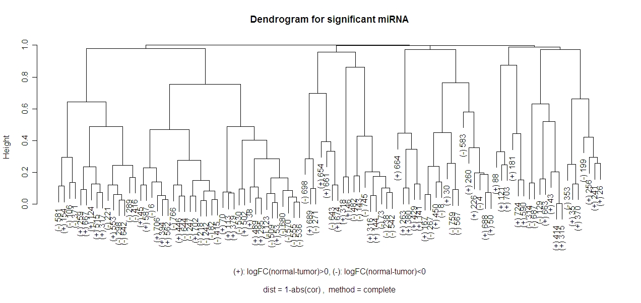
In this method it looks like there should be either 4 or 9 clusters.
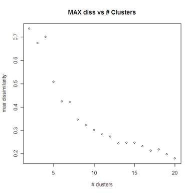
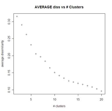
Using PAM for the number of clusters ranging from 2 to 20 we can see the average of the clusters’ max dissimilarity below left (the average dissimilarity is below right). For the max dissimilarity it looks like 8 clusters is the most appropriate number of clusters. There is no obvious elbow in looking at the average dissimilarity L plot below right.
|
|
|
Looking at the average silhouette widths compared to the number of clusters, we again see a clear jump when we get to 8 clusters (the bolded point). The average silhouette width is also large for 3 clusters, but looking at the dissimilarities above we see that 3 clusters is not very good. Although the maximum average silhouette width from 2 to 20 clusters is at 19 clusters, we do not want to say that there are that many clusters because that is much more complicated than we can accurately predict (especially only looking at 100 miRNA instead of all of them).
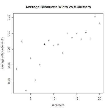
Because 9 and 13 clusters are both better than 8 in terms of lower dissimilarities and higher average silhouette width, these are other numbers of clusters that we might consider. So the numbers of clusters to consider are 8, 9, and 13.
>
clus8<-pam(rna.sig.dists,8)$clustering
>
clus9<-pam(rna.sig.dists,9)$clustering
>
clus13<-pam(rna.sig.dists,13)$clustering
>
>
table(clus8,clus9)
clus9
clus8 1
2 3 4
5 6 7
8 9
1 29
0 0 0
0 0 0
0 0
2
0 4 0
0 0 0
0 3 0
3
0 0 7
0 0 0
0 0 0
4
0 0 0 10
0 0 0
0 0
5
0 0 0 0
17 0
0 0 0
6
0 0 0
0 0 9
0 0 0
7
0 0 0
0 0 0 13
0 0
8
0 0 0
0 0 0
0 0 8
Comparing 8 and 9 clusters we see that the only difference is that in clus8, the second cluster gets split in half to make the new cluster for clus9.
>
table(clus8,clus13)
clus13
clus8 1
2 3 4
5 6 7
8 9 10 11 12 13
1 12
1 10 0 5
0 1 0
0 0 0
0 0
2
1 0 0
0 0 0
0 0 0
3 0 0 3
3
0 0 1
0 0 0
0 6 0
0 0 0 0
4
0 0 3
7 0 0
0 0 0
0 0 0 0
5
2 1 0
0 0 12 2
0 0 0
0 0 0
6
0 2 0
0 0 0
2 0 0
0 5 0 0
7
1 1 0
0 0 0
0 0 11 0
0 0 0
8
0 0 0
0 1 0
0 0 0
0 0 7 0
Going from 8 to 13 clusters there are many more changes. For example, the new cluster 2 in clus13 is made from 4 different clusters of clus8, and cluster 7 in clus13 is made out of 3 different clusters from clus8.
>
table(clus9,clus13)
clus13
clus9 1
2 3 4
5 6 7
8 9 10 11 12 13
1 12
1 10 0 5
0 1 0
0 0 0
0 0
2
1 0 0 0
0 0 0
0 0 0
0 0 3
3
0 0 1
0 0 0
0 6 0
0 0 0 0
4
0 0 3
7 0 0
0 0 0
0 0 0 0
5
2 1 0
0 0 12 2
0 0 0
0 0 0
6
0 2 0
0 0 0
2 0 0
0 5 0 0
7
1 1 0
0 0 0
0 0 11 0
0 0 0
8 0 0
0 0 0
0 0 0
0 3 0
0 0
9
0 0 0
0 1 0
0 0 0
0 0 7 0
Comparing 9 and 13 clusters we see that breaking up the original cluster 2 from clus8 (which went to cluster 2 and cluster 8 in clus9) stayed nearly the same – only one of those 7 points went into a third group when going to 13 clusters.
One clear difference between the smaller numbers of clusters (in clus8 or clus9) and the 13 clusters (in clus13) is that cluster 1 from clus8 (which is the same in clus9) is broken into 5 different clusters in clus13. The majority of the points from cluster 1 in clus8 and clus9 went into three main clusters in clus13 forming the majority of the clusters 1, 3, and 5 (respectively with size 12, 10, and 5).
>
adjrand(clus8,clus9)
[1]
0.9907233
>
adjrand(clus8,clus13)
[1]
0.4720343
>
adjrand(clus9,clus13)
[1]
0.4784161
The Adjusted Rand index also suggests that 8 and 9 clusters are very similar whereas 8 and 13 or 9 and 13 clusters are not as similar.
Given the dendrogram at the top of this page, I believe that 9 clusters is the right number of clusters. Using PAM to determine the clusters, we see that this matches the above dendrogram. (This is the exact same image except the gene name is replaced by which cluster it was put in). I have included the same dendrogram below replacing miRNA indices with the cluster that PAM put them into.
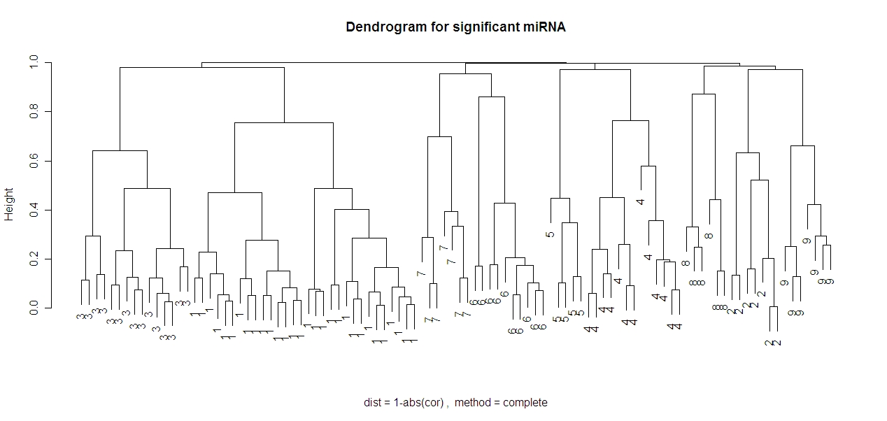
Note that the clusters match the obvious clusters from the dendrogram! Both the PAM method and the complete (hierarchical) method used the same distance metric of 1-abs(cor). This means that using the PAM method results in the same clusters as the complete method. This suggests that these clusters are not random, but rather represent clusters of miRNA that are truly co-expressed.
This website was designed by Austen Head.
Email: austen
[dot] head [at]