This web page was produced as an assignment for a course on
Statistical Analysis on Microarray Data at
NOTE THAT BEFORE BEGINNING THIS SECTION I HAD TO CHANGE THE “toReadIn.txt” FILE.
I have changed data info part also to include the change.
The only change is in the last two columns which I titled “Cy3” and “Cy5” to be able to use the R-package function modelMatrix() correctly to save me from some additional code.
In this section I am trying to determine which miRNA seem to most strongly distinguish between the several specific different types of tissue. Note that it might also be interesting to try to distinguish between healthy and unhealthy tissue but I decided not to do this because one thing that I thought was interesting in the study is that they realized that two of the samples that they used had originally been misdiagnosed. An ARMS was originally misdiagnosed as an ERMS (array 12 – in the data that was posted online the original researchers had already corrected this misdiagnosis so my arrays are correctly diagnosed), and a PRMS that was misdiagnosed as a GIST (array 22).
There are 1536 spots on each chip. Each miRNA is printed two times per chip (NOT randomly, but instead one print is exactly a Y Grid Coordinate within sector difference of 3). If two miRNA are in the same sector and their X Grid Coordinate (Xcoord) within sector is the same and their Ycoord is difference is 3, then it is actually the same miRNA.
################################
To distinguish ARMS and ERMS we can look at each of the 1536 spots individually and do a t-test on each one of those miRNA. There are 3 ARMS arrays (11, 12, 14) and 1 ERMS array (13).
So for the t-tests on spot j (where j=1,2,…,1536) we have the hypotheses:
H0: true mean expression of the miRNA at spot j for ERMS – true mean expression of the miRNA at spot j for ARMS = 0
Ha: true mean expression of the miRNA at spot j for ERMS – true mean expression of the miRNA at spot j for ARMS ≠ 0
Since we are performing 1536 t-tests, we do not want a high alpha like 0.10 because then even if the null hypothesis were true then we would still find 153 significant miRNA. So instead if we have alpha=0.01 and look at the adjusted p values of each of the 1536 t-tests, we see that there are 9 miRNA that are significant (this is still a very small number, but with so few ARMS and ERMS arrays it should not be too surprising). Below are the t-tests on miRNA which have the ten highest “log odds” (B values).
NOTE: the data that the researchers gathered from the arrays were generated by standardized software which automatically labeled the miRNA as “genes” instead of miRNA. Hence, below in the table, “gene” is actually miRNA.
|
Spot |
Gene.Symbol |
Gene.Name |
Sequence.Type |
X.Grid.Coordinate within.sector. |
Y.Grid.Coordinate within.sector. |
Sector |
logFC |
AveExpr |
t |
P.Value |
adj.P.Val |
B |
|
|
884 |
NA |
NA |
ss_oligo |
4 |
3 |
19 |
-3.40824 |
7.358119 |
-5.90269 |
3.13E-06 |
0.002443 |
4.582617 |
a |
|
908 |
NA |
NA |
ss_oligo |
4 |
6 |
19 |
-3.43729 |
7.312997 |
-5.80691 |
4.02E-06 |
0.002443 |
4.352503 |
a |
|
197 |
NA |
NA |
ss_oligo |
5 |
1 |
5 |
5.487415 |
8.443424 |
5.49623 |
9.04E-06 |
0.003554 |
3.60051 |
b |
|
1156 |
NA |
NA |
ss_oligo |
4 |
1 |
25 |
2.353148 |
8.462062 |
5.354102 |
1.17E-05 |
0.003554 |
3.351133 |
c |
|
545 |
NA |
NA |
ss_oligo |
1 |
3 |
12 |
4.429081 |
7.394094 |
5.238089 |
1.60E-05 |
0.003881 |
3.061908 |
d |
|
194 |
NA |
NA |
ss_oligo |
2 |
1 |
5 |
3.226374 |
6.517701 |
5.043222 |
3.31E-05 |
0.006495 |
2.40603 |
|
|
569 |
NA |
NA |
ss_oligo |
1 |
6 |
12 |
4.278728 |
7.391754 |
4.921453 |
3.74E-05 |
0.006495 |
2.270308 |
d |
|
1415 |
NA |
NA |
ss_oligo |
7 |
3 |
30 |
-1.74033 |
6.74557 |
-4.72978 |
6.82E-05 |
0.009734 |
1.72199 |
|
|
221 |
NA |
NA |
ss_oligo |
5 |
4 |
5 |
4.931103 |
8.429364 |
4.708998 |
7.20E-05 |
0.009734 |
1.670885 |
b |
|
1180 |
NA |
NA |
ss_oligo |
4 |
4 |
25 |
2.371478 |
8.385921 |
4.580213 |
9.36E-05 |
0.011175 |
1.416722 |
c |
As I mentioned earlier, these micorarrays have spot duplicates. We can see that the top two B values for miRNA are actually the same miRNA (marked a in the last column that I added), just duplicates (similarly with the third and ninth, and similarly with the fourth and tenth, and similarly with the fifth and seventh most significant miRNA). That suggests that those miRNA which have both their spots significant are useful miRNA in distinguishing between ERMS and ARMS tumors.
Unfortunately in the data none of the data has a name or symbol, the researchers put that identifying information in a column named “Reporter Name” which does not show up using the standard functions in the limma package of R. I tried to redo my line of code
full.dat<-read.maimages(dat.targets$Name,source="smd",wt.fun=dat.filter)
so it would include the reporter name, but doing that without messing up later code seems to be much more difficult to figure out than I would have guessed. It might be easier to simply cross reference the spot numbers (above in the table) with the reporter name from one of the datasets. Every miRNA on each chip is “ss_oligo” or “unknown” so that knowing that it’s an “ss_oligo” is not very useful.
For the miRNA that I marked with a, b, d, both spots are statistically significant at the 0.01 level and the log odds are greater than 1, so there is at least one fold difference between the miRNA on ERMS and ARMS arrays (so there is probably enough of a difference between the means of the a, b, d, miRNA to be biologically significant). So for a, b, d, we reject the null hypothesis H0 and we also believe that they are biologically significant miRNA. This suggests that the a, b, d miRNA can help discriminate between ERMS and ARMS tumor tissue types.
Volcano Plot of the spots (recall 2 spots per miRNA) comparing ARMS and ERMS:
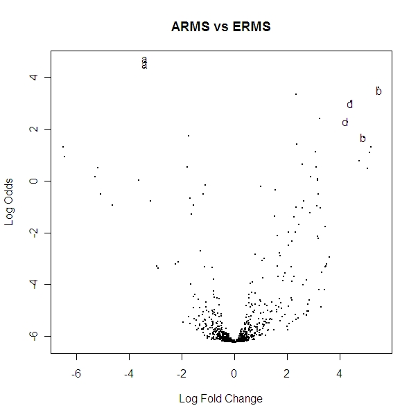
A volcano plot gives a visualization of the important information from the above table. The 10 highest points (on the Y axis) are the ones with the 10 highest B values (which are listed in the table above). I labeled the spots that I said are significant above. A volcano plot tells you what the log odds versus log fold change is for spots on the microarray. So look at the two points labeled “a” in the table: the logFC column gives the X axis (about -3.5) for both “a”s, the B column gives the Y axis (about 4.4). We expect to see very few points having a high log odds value where the log fold change is nearly 0 because when log fold change is near 0 that means there is not much biological significance at all, so we expect to see log odds to be low here.
################################
Doing nearly the exact same thing with PRMS and GIST with similar t-test hypotheses (replace ERMS with PRMS and replace ARMS with GIST) and following the same procedure we can get a table of the miRNA with the top ten log odds values (B values). There are 8 GIST arrays (1, 2, 5, 6, 21, 23, 24, 25) and 2 PRMS arrays (15, 16).
|
Spot |
Gene.Symbol |
Gene.Name |
Sequence.Type |
X.Grid.Coordinate within.sector. |
Y.Grid.Coordinate within.sector. |
Sector |
logFC |
AveExpr |
t |
P.Value |
adj.P.Val |
B |
|
|
1137 |
NA |
NA |
ss_oligo |
1 |
5 |
24 |
4.753428 |
8.845317 |
8.033913 |
1.22E-08 |
1.48E-05 |
9.815962 |
a |
|
1113 |
NA |
NA |
ss_oligo |
1 |
2 |
24 |
4.61066 |
8.841657 |
7.427744 |
5.37E-08 |
3.26E-05 |
8.43079 |
a |
|
607 |
NA |
NA |
ss_oligo |
7 |
4 |
13 |
-5.65734 |
11.39965 |
-5.92134 |
2.58E-06 |
0.000881 |
4.777492 |
b |
|
583 |
NA |
NA |
ss_oligo |
7 |
1 |
13 |
-5.57109 |
11.5787 |
-5.8774 |
2.90E-06 |
0.000881 |
4.667249 |
b |
|
737 |
NA |
NA |
ss_oligo |
1 |
3 |
16 |
-4.27701 |
7.475112 |
-5.46218 |
8.75E-06 |
0.001401 |
3.61841 |
c |
|
761 |
NA |
NA |
ss_oligo |
1 |
6 |
16 |
-4.37404 |
7.32241 |
-5.45809 |
8.85E-06 |
0.001401 |
3.608045 |
c |
|
1277 |
NA |
NA |
ss_oligo |
5 |
4 |
27 |
4.746537 |
12.11954 |
5.446828 |
9.12E-06 |
0.001401 |
3.579437 |
d |
|
1253 |
NA |
NA |
ss_oligo |
5 |
1 |
27 |
4.702163 |
12.03123 |
5.442931 |
9.22E-06 |
0.001401 |
3.569541 |
d |
|
993 |
NA |
NA |
ss_oligo |
1 |
5 |
21 |
-4.63833 |
11.54595 |
-5.09194 |
2.36E-05 |
0.003193 |
2.675746 |
|
|
545 |
NA |
NA |
ss_oligo |
1 |
3 |
12 |
-2.84123 |
7.394094 |
-4.9079 |
3.88E-05 |
0.004422 |
2.206044 |
|
As with the comparison between the ERMS and ARMS we see that there are 4 miRNA where both spots have very high log odds (marked a through d above). There are more B values that are high in this comparison between GIST and PRMS than there were between ERMS and ARMS. This is not too surprising since there are a lot more arrays between the GIST and PRMS than there were between the ERMS and ARMS.
For the miRNA that are represented by the spots that I marked a, b, c, d, we can reject H0 and also see that the B values are large enough that their difference is biologically significant. There are probably other miRNA between PRMS and GIST that are both statistically significant and biologically significant, but I am only showing the top ten B values for the 1536 miRNA. This suggests that the a, b, c, d miRNA can help discriminate between the PRMS and GIST tumor tissue types.
Volcano Plot of the spots (recall 2 spots per miRNA) comparing PRMS and GIST:
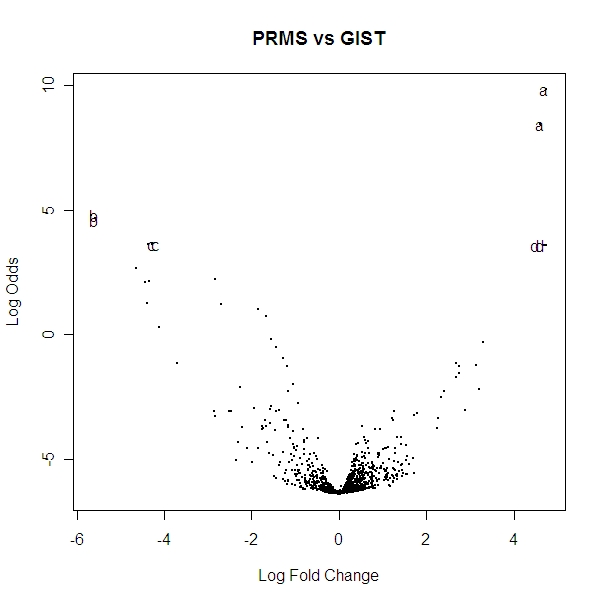
I again marked a, b, c, d on the above plot corresponding to the miRNA mentioned above. The volcano plots shows that the two spots for each a, b, c, d are very close together which is what we expect to see since they are the same miRNA and there are enough samples of each of these to be relatively reliable. These do in fact look like they are the most significant points also which indicates that these are probably good miRNA to help distinguish PRMS and GIST tumors.
##############################################################################################
MODIFIED APRIL 11
I have since redone this section to combine spots for single miRNA. I am not going to do analysis again, but I am mainly doing this to compare limma to SAM for the following section.
ARMS vs ERMS
 > dat.topTable1
ID logFC t
P.Value
adj.P.Val B
580
2.362313 5.215328 1.722599e-05
0.006261658 2.98417074
281 ambi_miR_13237 4.353904
5.155586 2.021610e-05 0.006261658
2.83704244
101 hsa_miR_380_5p 5.209259
5.098591 2.612653e-05 0.006261658
2.61102860
255
5.164235 4.496471 1.184716e-04
0.016822294 1.21026627
699
-6.471218 -4.541632 1.341436e-04 0.016822294 1.12733516
452 ambi_miR_10766 -3.422761
-4.433075 1.403808e-04 0.016822294
1.05417508
551 ambi_miR_10394 2.983464
4.303697 1.983493e-04 0.017607661
0.73631674
719
-1.760304 -4.264754 2.200562e-04 0.017607661 0.64085980
513
4.889119 4.264165 2.204019e-04
0.017607661 0.63941722
185 hsa_miR_202 -5.242502 -4.195862 2.643691e-04
0.019008139 0.47228601
360 ambi_miR_10133 3.128503
4.136507 3.095481e-04 0.020233193
0.32738866
605 hsa_miR_383 -1.160560 -4.077705 3.834236e-04
0.022973467 0.14020218
206
2.585193 3.971231 4.794928e-04
0.026519640 -0.07413443
541 hsa_miR_495
3.173087 3.903489 5.732123e-04
0.029187625 -0.23773842
561
-3.416367 -3.880511 6.089212e-04 0.029187625 -0.29308924
61
-1.628324 -3.737273 8.861101e-04 0.039819575 -0.63630603
755
-4.862694 -3.724741 9.578497e-04 0.040511409 -0.69883851
628 hsa_miR_505
3.205249 3.595408 1.280996e-03
0.051168668 -0.97272369
438 2.480831 3.436091 1.929671e-03 0.073022826 -1.34562404
608 hsa_miR_525
2.303134 3.416070 2.184385e-03
0.078528649 -1.44196244
57 hsa_miR_515_3p
1.578324 3.339619 2.466984e-03
0.084464818 -1.56854578
738 hsa_miR_155
1.124161 3.256397 3.243679e-03
0.106009330 -1.80089788
179 hsa_miR_519d
2.313546 3.183628 3.653858e-03
0.112321685 -1.92378538
627 hsa_miR_10b 3.316390 3.173309 3.749263e-03 0.112321685 -1.94703911
729 2.046726 3.174092 3.968903e-03 0.114145644 -1.98347916
PRMS vs GIST
 > dat.topTable2
ID logFC t
P.Value
adj.P.Val B
561
4.682044 7.767644 2.409615e-08
1.732513e-05 9.1487042
295
-5.614216 -5.892516 2.840995e-06 1.021338e-03 4.6865056
377 hsa_miR_133b -4.325524 -5.452137 9.145727e-06
1.703807e-03 3.5837442
629 hsa_miR_517a
4.724350 5.438734 9.478757e-06
1.703807e-03 3.5499855
489
-4.537370 -4.995085 3.109170e-05 4.470987e-03 2.4285694
281 ambi_miR_13237 -2.768114
-4.787540 5.427438e-05 6.503880e-03
1.9028109
337 CONTROL_30
-4.356353 -4.493485 1.194229e-04 1.226644e-02
1.1593276
306 hsa_miR_410 -3.908199 -4.116466 3.264630e-04
2.934086e-02 0.2136053
602
-1.359085 -3.769650 8.142714e-04 5.949799e-02 -0.6420940
185 hsa_miR_202
3.219419 3.763478 8.275103e-04
5.949799e-02 -0.6571495
198 hsa_miR_522
2.717738 3.687496 1.008807e-03
6.593931e-02 -0.8419334
370 hsa_miR_128a
2.718155 3.364578 2.315514e-03
1.387379e-01 -1.6134855
274
-1.057676 -3.332621 2.511140e-03 1.388854e-01 -1.6884511
586
-1.351366 -3.099706 4.902866e-03 2.478820e-01 -2.2584592
359 ambi_miR_3121
2.380840 3.043620 5.171391e-03
2.478820e-01 -2.3527113
392 hsa_miR_199b
1.166790 3.021171 5.914288e-03
2.531927e-01 -2.4302649
731
-3.455706 -3.027163 6.428850e-03 2.531927e-01 -2.4993519
91 ambi_miR_9630 -0.926332 -2.956845 6.396282e-03 2.531927e-01
-2.5468041
699
3.043015 2.947477 7.042913e-03
2.531927e-01 -2.5733034
437 hsa_miR_148a -1.749784 -2.936506 6.720900e-03 2.531927e-01
-2.5919020
120 ambi_miR_11143 -3.151130
-2.827866 1.010229e-02 3.301613e-01 -2.8742912
588
-1.567868 -2.807455 9.173775e-03 3.140926e-01 -2.8743584
657 hsa_miR_377 -2.486712 -2.725752 1.113972e-02 3.482373e-01
-3.0497097
259 ambi_miR_11576 1.762352
2.686120 1.222980e-02 3.576332e-01 -3.1337435
492
-2.842451 -2.683084 1.253223e-02 3.576332e-01 -3.1496578
This website was designed by Austen Head.
Email: austen [dot] head [at]