Hilary Parker | Math 155 Project

This web page was produced as an assignment for a course on Statistical Analysis of Microarray Data at Pomona College.

Hierarchical Clustering:
To examine the effectiveness of hierarchical clustering, we performed clustering on two subset of miRNAs - 20 random miRNAs, and 20 significant ones.

Random miRNAs:
R was used to select 20 random indices from our total, merged miRNA data (768 miRNAs possible). Presumably, there is no relationship between these miRNAs, so that any clustering observed is just a remnant of the fact that hierarchical clustering always must create clusters, even when they are not significant.

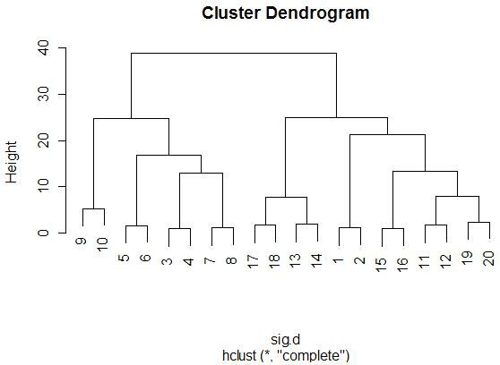
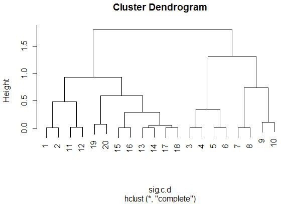
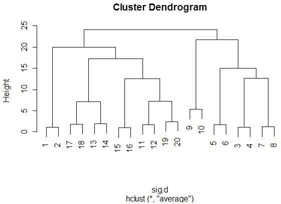
Below are dendrograms from the clustering. Below each dendrogram is a brief explanation of both the distance method and clustering method used. Note that the heights of the trees differ because they are a direct reflection of the linkage and distance methods used. So, for example, because 1-correlation yields a maximum distance of 2, we would not expect the trees to get any higher than 2. Likewise, complete linkage (which measures cluster distances based on the farthest elements) will yield much higher trees than average linkage (which measures cluster distances based on the average of all the elements).

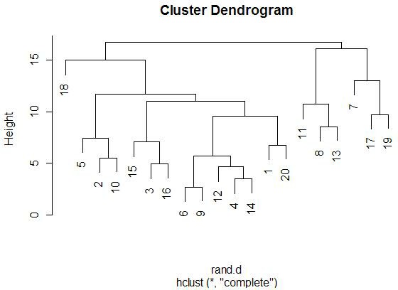
Clustering using Euclidean distance and complete linkage method (distance between clusters is measured according to the farthest cluster elements).	Clustering using 1-correlation as distance and complete linkage method.
Clustering using Euclidean distance and average linkage method (distance between clusters is measured according to the averaged values of the cluster elements).	Clustering using 1-correlation distance and average linkage method.

With the graphics above, it is meaningful to compare the graphs that are both side-by-side, as well as top-and-bottom. Side-by-side trees use the same linkage method, and top-and-bottom trees use the same distance method.

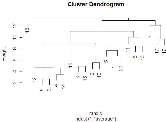
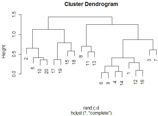
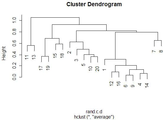
Interestingly, the euclidean distance trees clustered with average and farthest methods both retain some of the same clusters (7-17-19, 11-13-8). Similarly, for the 1-correlation distance trees, the clusters are all somewhat similar, especially pair-wise clusterings (17-19, 15-18, 12-16). This makes sense because the farthest element heavily influences the average calculation (since the average is not robust). So, these results make sense).

Comparing the same linkage methods with different distance methods (side-by-side comparisons) yields less similarity between the clusters. The general location of the different miRNAs is somewhat retained, but we see less similar clusters and less similar pairings.

When comparing caddy-corner from one another, we again see a decrease in similarities. One notable exception is the 8-11-13 cluster, which appears in three of the four trees. These miRNAs must be very similarly expressed in both magnitude (Euclidean measure) and trend (correlation measure). We also see 17-19 paired together in every tree, with the same interpretation.

Significant miRNAs:
Because the previous analyses were done with the uncompressed data (that is, the spots were not merged), I decided to do this analysis with the uncompressed data as well. It actually affords an interesting control, because spots that are the exact same miRNA should cluster together no matter what.

Below is a table of the significant genes used:

Spot Number	miRNA name
1146	hsa_miR_122a
1122	hsa_miR_122a
993	hsa_miR_145
969	hsa_miR_145
75	hsa_miR_29b
51	hsa_miR_29b
523	ambi_miR_7510
499	ambi_miR_7510
197	hsa_miR_214
221	hsa_miR_214
1421	hsa_miR_422b
1397	hsa_miR_422b
1499	hsa_miR_1
1523	hsa_miR_1
695	(blank)
719	(blank)
1419	hsa_miR_133a
1395	hsa_miR_133a
1448	hsa_miR_422a
1472	hsa_miR_422a

Below are dendrograms from the clustering. Below each dendrogram is a brief explanation of both the distance method and clustering method used.

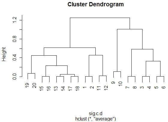
Clustering using Euclidean distance measurements and complete linkage (distance between clusters is defined by distance between farthest elements of each cluster).	Clustering using 1-correlation distance measurements and complete linkage.
Cluster using Euclidean distance method and average linkage method (distance between clusters is measured according to the averaged values of the cluster elements)	Clustering using 1-correlation distance method and average linkage method.

There are a few things to note from these diagrams. First, happily, all of the neighbors (1-2, 3-4, 5-6, etc.) represent the exact same miRNA, so it's a good thing that they are all clustering together first.

When we take a step back and look at the larger clusters (realizing that the pairwise ones can be considered one group), we see some similarities between all of the clustering techniques. The cluster (3-4-5-6-7-8-9-10) appears in all four trees as a highly isolated branch. In fact, this can be taken one step further to say that each tree divides into two main clusters - the one just described and then the left-overs.

When looking at smaller clusters, we see more similarities between all four trees. One obvious one is the cluster (13-14-17-18), which appears in all four trees as closely linked. Several times, there are clusters that contain the same elements but are just paired up in a different order, such as (3-4-5-6-7-8-9-10). Interestingly, in this case, (3-4) links first to (7-8) when using Euclidean distance, but when using 1-correlation distance, (3-4) links first to (5-6).

Comparing these results to the random miRNA results shows that these results are much more consistent across different distance and linkage methods. One might go so far as to say that one should use multiple clustering methods before determining that a cluster is significant. Because hierarchical clustering always results in a tree, it seems like a good way to check if your tree is significant is to calculate it multiple ways and see if it remains the same. In our case, anyway, we would quickly be able to determine which trees are from the random miRNAs and which are from the significant ones.