HOME |  DESIGN |  MICROARRAY SAMPLES |  NORMALIZATION |  SIGNIFICANCE TESTING |  SAM |  H. CLUSTERING |  PAM CLUSTERING |  PAM CLASSIFICATION |  CONCLUSIONS

This web page was produced as an assignment for a course on Statistical Analysis of Microarray Data at Pomona College.

PAM Clustering:
Because of the small size of the dataset, I was able to perform PAM clustering on the entire miRNA library (768 genes total).

There are two k-values we are interested in biologically:  k=2 (healthy versus tumor tissue) and k=9 (because there are 7 tumor types and 2 healthy tissue types).  However, we will compute PAM clusters for several k-values to compare the results.

Two separate distance metrics were used - Pearson correlation and Euclidean distance.

Silhouette Width:
Below is a summary of the Silhouette widths for PAM clusterings at various k-values using distances based on Pearson correlation as well as Euclidean distance. Note that silhouette widths close to 1 are desired.  Also note that for neither distance method does k=9 look like the optimal number of clusters.

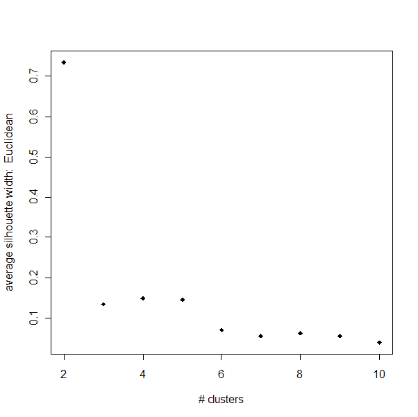
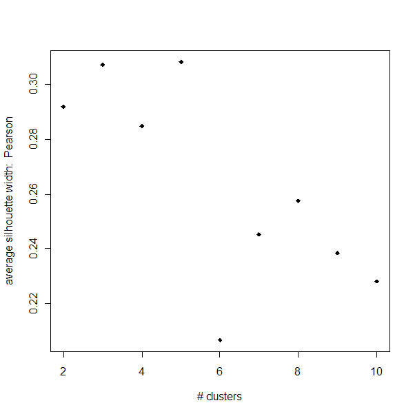
There are a couple of interesting things to point out.  Our strongest clusters are with Euclidean distances and k=2.  However, for k>2, the Euclidean clusters peform very weakly.  The Pearson clusters have consistantly higher silhouette widths than the Euclidean ones for k>2.  The Pearson clusters also have a more interesting pattern - for whatever reason, at k=6, the silhouette width drops drastically but then returns to stronger values instantly.  These results could indicate that k=9 clusters aren't ideal, perhaps because some of the tumor types are extremely similar in expression profiles.

Maximum Dissimilarity:
The maximum dissimilarity is a measure of the maximum distance between two members of one group.  It will continue to decrease until k=n (number of miRNAs), but it does level off significantly when the clustering is saturated.

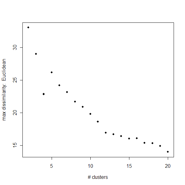
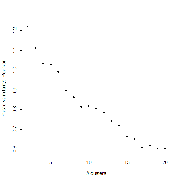
There is a clear "elbow" to the Euclidean distance dissimilarities around k=11.  For the Pearson dissimilarities, the elbow is not as clear, but could occur as late as k=17.

Tables
Comparing the clusters of the Euclidean versus Pearson can add insight into which clustering method is more appropriate.  Below is a comparison of the Euclidean versus Pearson clustering for k=9.  The rows are Pearson clusters, and the columns are Euclidean clusters.



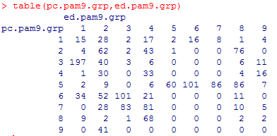
The Pearson cluster #1, and perhaps #2, are evenly spread out between the 9 Euclidean clusters, but after that the Pearson clusters seem to correlate to certain subsets of the Euclidean clusters.  The Euclidean clusters seem to be spread out among the Pearson clusters more consistently, with only #5, #6, #7 and perhaps #3 showing any specificity.

Discussion
It's difficult to determine whether or not the clusters we have are in fact legitimate.  I give much more weight to the Pearson correlation distances than the Euclidean distances for this analysis.  Thus, the low silhouette widths are discouraging for k=9.  However, for 1<k<5, the silhouette widths are somewhat acceptable, so it might be worth investigating whether some of the tumor types have very similar expression profiles (and thus cluster together).  I also want to investigate the two clusters found using the Euclidean distance method to see if they correlate to tumor versus healthy tissues.

The authors used hierarchical clustering methods, so this PAM analysis would be completely new.