|
HOME | DESIGN | MICROARRAY SAMPLES | NORMALIZATION | SIGNIFICANCE TESTING | SAM | H. CLUSTERING | PAM CLUSTERING | PAM CLASSIFICATION | CONCLUSIONS |

This web page was produced as an assignment for a course on Statistical
Analysis of Microarray Data at
The normalization procedure used in this project was the Loess method, which is
a Robust regression method. With user-specified parameters, the algorithm for
normalization is basically a series of weighted linear regressions over a small
subset of the data, repeated many times and smoothed to create a best-fit line.
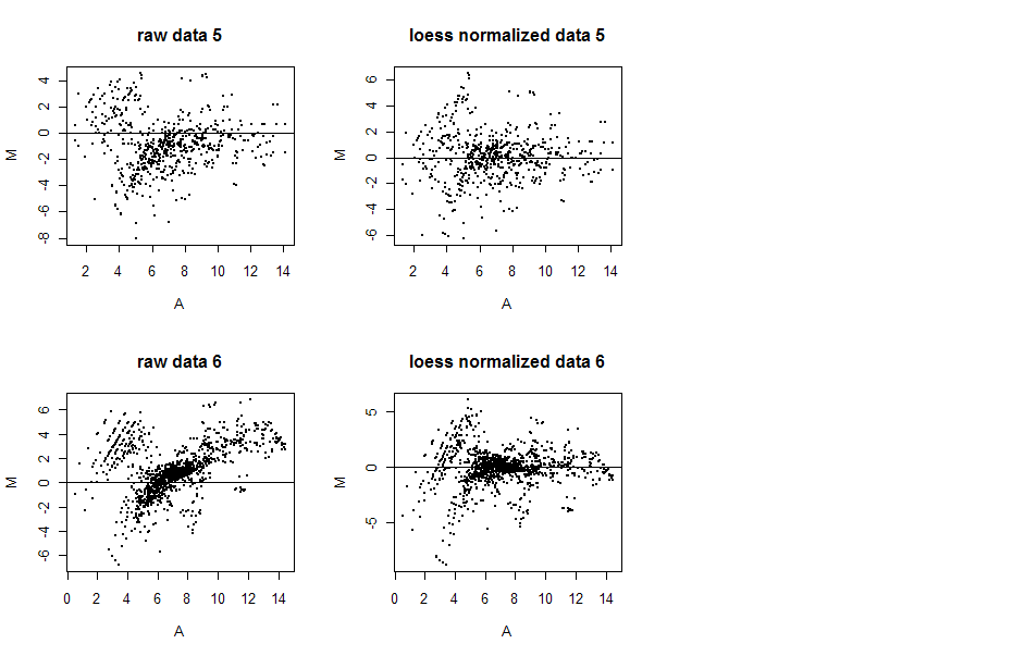
The MA plots below display data before and after loess normalization for two
arrays (5 and 6). In the case of loess plots, the M's for each A-value are
determined using the loess fit described above. Notice how in both cases, after
normalization the data appear to be centered over the M=0 line, but not before.
This is especially apparent in array 6, where a significant positive trend is
essentially erased with normalization.
Boxplots for each of the arrays before and after normalization are displayed
below.
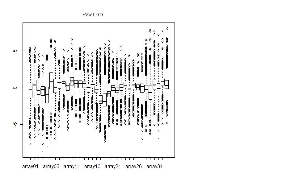
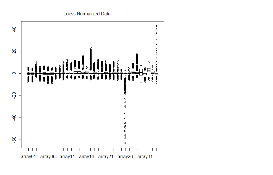
Note that the y-axis is quite different for each plot. Arrays 26 and 34 look as
though normalization actually skewed the data more, although MA plots do not
indicate such a drastic change in M-values.
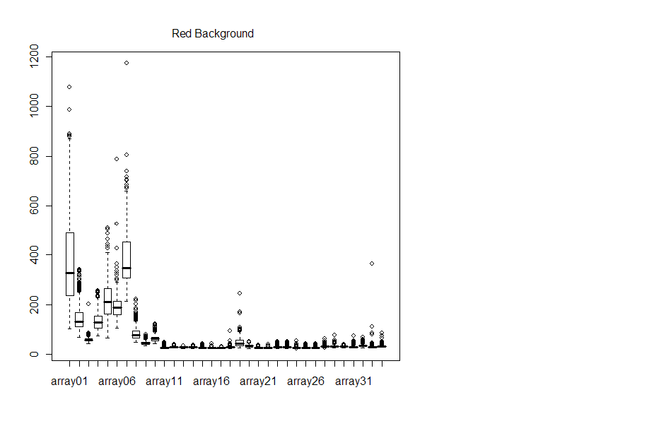
Boxplots of the background confirm what we saw visually with the microarray chip - the background data is very noisy.

Next, normalization was tested two ways (Kolmogorov-Smirnov method and Looney
and Gulledge method).
Using 50 randomly selected genes, the following p-values were obtained using
the KS method:
0.177828
0.02952348*
0.5625915
0.516381
0.1233222
0.2360967
0.34369
0.09966977
0.1853652
0.3020463
0.04049711*
0.0702582
0.00320633*
3.040773e-05*
0.1848228
0.9039434
0.1461928
0.02026443*
0.03136127*
0.8024172
0.006344712*
0.5064732
0.1773753
0.6533653
0.1195844
0.009225614*
0.1996645
0.01036490*
0.5589412
0.675567
0.8987557
0.03379657*
0.1580227
0.0372678*
0.7973501
0.1790031
0.1819115
0.7938111
0.4737908
0.5437275
0.09287292
0.01194443*
0.06556916
0.004963614*
0.2068782
0.6062126
0.1652469
0.01839006*
0.07193951
0.2956484
Samples with stars are significant at the 0.05 level, indicating that we can
reject the null hypothesis that they are normal. Note that we would expect
approximately 2-3 type I errors in 50 samples, but we have 14. This may suggest
that our data is not reliably normalized.
The next test for normality was the Looney & Gulledge test of normality,
which finds the correlation coefficient of the qq-plot of normal quantiles and
determines its significance. The correlations are listed below. Note that 34
arrays were used in total, so at a 0.05 level, the critical value from a Looney
table is 0.968. Stars are placed next to values that are significantly
different from normal.
0.907135*
0.7911997*
0.8533497*
0.9820423
0.9657144*
0.9847417
0.8433906*
0.95118*
0.7972965*
0.9397885*
0.8361207*
0.9109652*
0.914329*
0.9211378*
0.8658665*
0.9493248*
0.920989*
0.9527418*
0.8242175*
0.8843698*
0.9065188*
0.756679*
0.7891022*
0.9142712*
0.848973*
0.9721124
0.9738254
0.9534558*
0.9300567*
0.7930633*
0.883229*
0.6168813*
0.9860473
0.774802*
0.901778*
0.9948245
0.7889048*
0.941132*
0.7807806*
0.740908*
0.819511*
0.9040048*
0.7649094*
0.9756437
0.7799284*
0.9495617*
0.9864484
0.9088602*
0.7422973*
0.9724674
Clearly, most genes fail the qq-plot test for normality. One factor that was
not taken into consideration is that for some of the genes above, they may have
had "NA" entries in one or more of the arrays. As such, a different
critical value should be used for them. However, an efficient means to find these
critical values was not known by me.